3346
Can eddy currents and concomitant fields be compensated at the same time in flow-compensated diffusion MRI?1Medical Physics in Radiology, German Cancer Research Center, Heidelberg, Germany, 2Institute of Radiology, University Hospital Erlangen
Synopsis
The possibility to simultaneous compensate for flow, concomitant fields and eddy currents in diffusion weighted MRI were examined by means of numerical simulations. For this purpose, sequences with three to five gradient pulses and one or two refocusing pulses were examined. It is shown that it is possible to effectively minimize all three effects with different sequences. For short to intermediate echo times, it is beneficial to use only one refocusing pulse, while for long echo times two refocusing pulses can yield higher b-values. There is a trade-off between compensation of more effects and the achievable b-value.
Purpose
For
diffusion encoding in MRI, high gradient amplitudes are needed, but the
application of strong gradient pulses induces artifacts resulting from eddy
currents and concomitant fields. Sequences that compensate for eddy currents in
non-flow-compensated diffusion MRI have been presented1. To our knowledge, however, flow-compensated
sequences that compensate for eddy currents and concomitant fields have not
been available so far, although the usefulness of flow-compensated diffusion
weighted imaging has been described in some recent works2,3. Thus, a numerical framework was
set up to search for solutions that maximize the b-value, while optionally
compensate flow, eddy currents and/or concomitant fields.Methods
Input parameters for the optimization were: gradient amplitude 40 mT/m, RF pulse duration 5 ms, duration of echo planar readout train before spin echo 10 ms. As shorthand notation for the diffusion encoding, a + or – sign is used to denote a gradient with positive/negative amplitude and the symbol | is used for a 180° RF pulse. The considered sequences consisted of three to five rectangular gradient pulses of identical amplitude and one or two refocusing RF pulses. Adjacent gradients needed to switch signs or be separated by a RF pulse (e.g. +–|–+ was considered but ++|– – was not). A sign change of all gradients yields essentially the same sequence, and so they were excluded from consideration. For the optimization, the gradient durations ($$$d_i$$$) and the times between the time between gradients ($$$t_i$$$) were varied. $$$d_i=0$$$ was allowed. To limit the number of gradient profiles further, only the sequences, that can possibly compensate for concomitant fields were taken into account, as this was fairly easy to verify under the assumption of gradient reversal. The gradient reversal was enforced by fixing the first gradient duration such that:
$$\sum_i{s_i^{\prime}\,d_i}=0,$$
where $$$s_i^\prime$$$ stands for the effective sign of the gradient taking the inversions by 180° RF pulses into account.
In the case of two RF pulses, the echo time TE is determined by the separation of these two, which allows one to fix an additional timing parameter, which was chosen to be the time between the gradients ($$$t_3$$$). The actual distance of the first RF pulse to the excitation is in this case irrelevant for TE, which allows one to fix the total duration of the diffusion encoding to the maximal available time (TE - [time for excitation] - [time for EPI echo train until the actual echo]), without loss of generality, and with that an additional timing parameter ($$$d_2$$$). In the cases with only one RF pulse, these parameters cannot be fixed. Timing constraints were used to ensure that the RF pulse is at the specified time and the diffusion encoding is played out in the allowed time.
For flow-compensation, the first gradient moment needs to be nulled, where $$$t_{i,s}$$$ denotes the starting time of the i-th gradient:
$$m_1=\sum_i{s_i^{\prime}\left(\frac{\delta_i^2}{2}+\delta_i\,t_{i,s}\right)}=0.$$
The condition for concomitant field compensation can be written as:
$$\sum_i{s_i^{\prime\prime}\,\delta_i}=0,$$
where
$$s_i^{\prime\prime}=\begin{cases}+1,\;\text{if 0 or 2 RF pulses have been applied before gradient pulse}\\-1,\;\text{if 1 RF pulse has been applied before gradient pulse}\end{cases}.$$
As model for eddy currents, it was assumed that each change in gradient amplitude produces eddy currents proportional to it, which then decay exponentially with the decay time $$$\tau=70$$$ ms4,5. The condition to null eddy currents is thus:
$$\sum_i{s_i\left(\exp{\left(-\frac{T-t_{i,s}}{\tau}\right)}-\exp{\left(-\frac{T-\delta_i-t_{i,s}}{\tau}\right)}\right)}=0,$$
which has to be fulfilled, where $$$s_i$$$ gives the actual sign of the i-th gradient.
For the optimization, Matlabs Global Optimization Toolbox (The Mathworks, Naticks, MA) was used with the GlobalSearch algorithm, which uses stochastic seed points and a local minimizer to find the global minimum6. The different compensation conditions were used as constraints in the algorithm.
Results
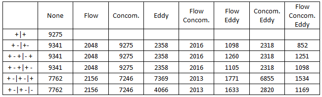
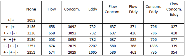
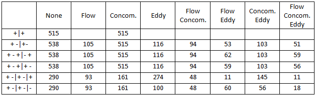
In Tables 1-3, the maximal b-values for each compensation are shown for three echo times for the sequences with the highest possible b-values while compensating all effects and for the standard Stejskal-Tanner-sequence (+|+). Since gradient durations are allowed to be zero, some sequences with nominal 5 gradients show the same optimal b-value as ones with 4.Discussion
The concurrent compensation of flow, eddy currents and concomitant field is possible, but it entails reduced b-values. The sequences with one RF pulse outperform those with two in most cases, because the additional pulse needs time. The important case of compensation of eddy currents1 is an exception to this rule.Conclusion
Depending on the actual study, it should be decided, which kind of compensation is needed, as there is a trade-off between b-value and compensating more artifacts.Acknowledgements
Financial support by the DFG (grant no. KU 3362/1-1 and LA 2804/2-1) is gratefully acknowledged.References
1. Reese TG, Heid O, Weisskoff RM, Wedeen VJ. Reduction of eddy-current-induced distortion in diffusion MRI using a twice-refocused spin echo. Magn Reson Med 2003;49(1):177-82.
2. Wetscherek A, Stieltjes B, Laun FB. Flow-compensated intravoxel incoherent motion diffusion imaging. Magnetic Resonance in Medicine 2015;74(2):410-419.
3. Ahlgren A, Knutsson L, Wirestam R, Nilsson M, Stahlberg F, Topgaard D, Lasic S. Quantification of microcirculatory parameters by joint analysis of flow-compensated and non-flow-compensated intravoxel incoherent motion (IVIM) data. Nmr in Biomedicine 2016;29(5):640-649.
4. Jezzard P, Barnett AS, Pierpaoli C. Characterization of and correction for eddy current artifacts in echo planar diffusion imaging. Magn Reson Med 1998;39(5):801-12.
5. Jehenson P, Westphal M, Schuff N. Analytical Method for the Compensation of Eddy-Current Effects Induced by Pulsed Magnetic-Field Gradients in Nmr Systems. Journal of Magnetic Resonance 1990;90(2):264-278.
6. Ugray Z, Lasdon L, Plummer J, Glover F, Kelly J, Marti R. Scatter search and local NLP solvers: A multistart framework for global optimization. Informs Journal on Computing 2007;19(3):328-340.
Figures