3284
Optimization of inversion-time sampling for precise estimation of renal perfusion with ASL1Department of Radiology and Imaging Sciences, University of Utah, Salt Lake City, UT, United States
Synopsis
This study outlines an approach for selecting optimal TIs at which to sample renal ASL data. We present an error-propagation factor for a model of the ASL signal and propose to optimize TI sampling through minimization of this factor. Using FAIR ASL data from 7 human subjects, we show that renal perfusion estimates obtained with optimal TI sampling are more accurate and precise than estimates obtained with uniform TI sampling, particularly when ASL data is acquired at only a few TIs.
Introduction
Acquiring ASL data at multiple inversion times (TIs) allows for better characterization of the ASL signal and more accurate perfusion estimation.1 For renal ASL, however, acquiring data at each TI typically requires a breath hold which can make multi-TI examinations difficult. In this study, we outline an approach for sampling TIs that maximizes the estimation-precision of ASL perfusion quantification, thereby enabling accurate estimation of renal perfusion from fewer acquisitions. We compare our proposed TI sampling method against uniform TI sampling, using flow-sensitive alternating inversion recovery (FAIR) ASL data from 7 human subjects.Theory
In FAIR ASL, subtraction of a nonselective inversion-prepared (NS) image from a slice-selective inversion-prepared (SS) image yields a signal-difference that is weighted by perfusion. This difference signal (dS) can be described by the following formula2:$$dS(TI)=\begin{cases}0\quad&TI<t_{0}\\S_{0}\cdot{}F\cdot{}(TI-t_{0})\cdot{}\exp(-TI/T_{1})\quad&TI\geq{}t_{0}\end{cases}\quad(1),$$where TI is the time-delay between inversion and image-acquisition, S0 is the difference signal immediately after inversion, F is perfusion, t0 is the transit-delay required for tagged blood to reach the imaging slice, and T1 is tissue T1. These parameters can be estimated by fitting equation 1 to multi-TI FAIR data. During this fitting, random noise (δ) in dS propagates into parameter estimates. An error-propagation factor ξ can be defined as the ratio of relative error in a model parameter to relative input noise3,4:$$\xi(n)=\frac{\delta{}x(n)/x(n)}{\delta{}/S_0}=\frac{S_0}{x(n)}\sqrt{\sum_{m=1}^{4}\sum_{p=1}^{4}\sum_{i=1}^{N_{TI}}\left[A^{-1}(n,m)\cdot{}A^{-1}(n,p)\cdot{}\frac{\partial{}dS(TI_{i},x)}{\partial{}x(m)}\cdot{}\frac{\partial{}dS(TI_{i},x)}{\partial{}x(p)}\right]}\quad(2).$$Here, x(n) (n=1,2,3,4) represents the parameters of equation 1: S0, F, t0, and T1, δx is the propagated parameter error, and A=JTJ where J is the Jacobian matrix of dS. ξ(n) is a function of NTI TIs, and can be minimized by adjusting the TI values using numerical optimization. Equation 2 can be generalized to the measurement of multiple parameters-of-interest that may vary for different tissues3:$$\overline{\xi}=\int_{F^{min}}^{F^{max}}\int_{t_{0}^{min}}^{t_{0}^{max}}\int_{T_{1}^{min}}^{T_{1}^{max}}(\xi_{T_1}+\xi_{t_0}+\xi_{F})\cdot{}dT_{1}dt_{0}dF\quad(3).$$Xmin to Xmax identifies the expected range of parameter X across tissues of interest, and ξx is the error-propagation factor for parameter X (equation 2). Minimizing equation 3 determines the TI values that minimize the propagation of error into the estimated parameters, i.e., that produce the most precise parameter estimates.Methods
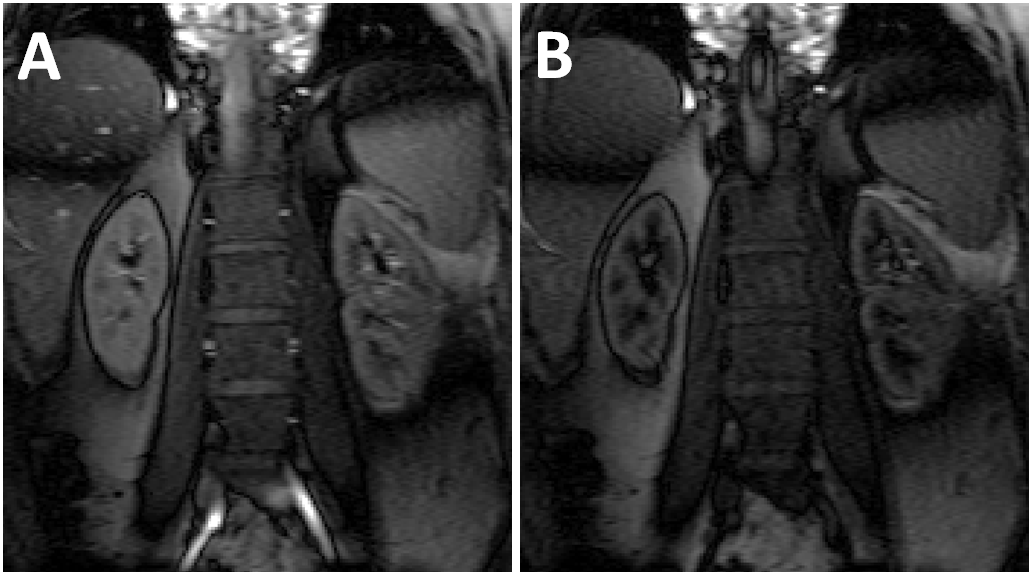
In this IRB-approved study, ASL data were acquired from 7 healthy volunteers at 3T (TimTrio; Siemens) using FAIR tagging and bSSFP readout: TR 3.68ms, TE 1.84ms, FOV 380×380mm, matrix 256×256, slice thickness 8mm, centric reordering, and GRAPPA factor 2. For each patient, data were acquired at 16 TIs: 150ms, then 200ms–1600ms at 100ms intervals. At each TI, SS and NS images were acquired at end-inspiration from a coronal slice through the kidneys (Figure 1).
SS and NS signal-versus-TI curves were obtained for each kidney by averaging the signal intensity within cortical and medullary ROIs on the SS and NS images at each TI. Subtraction of NS signals from SS signals yielded ASL difference-signal curves for each kidney. Reference perfusion measurements were obtained by fitting these 16-TI difference-signal curves with equation 1.
The 16-TI difference-signal curves were then downsampled to produce curves with 4 TIs and 8 TIs. The TIs included in the 4-TI and 8-TI curves were chosen from the original 16 using two strategies: 1) Uniform sampling, wherein TIs were uniformly distributed along the original curve, and 2) Optimized sampling, wherein TIs were determined by minimizing equation 3 and selecting TIs from the original 16 that most closely matched the optimal TIs from the minimization. Equation 3 was minimized over expected renal-parameter ranges: F: 150–650mL/min/100g, t0: 0–200ms, and T1: 800–2000ms.
Perfusion was estimated from the downsampled curves by fitting with equation 1. The accuracy of perfusion estimates from the downsampled curves was evaluated by computing the absolute difference between reference perfusion estimates and those from the downsampled curves (ΔF = |Freference – Fdownsampled|). Correlation between reference perfusion values and those from downsampled curves was also determined.
Results
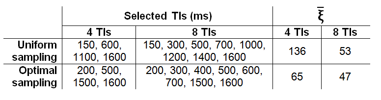
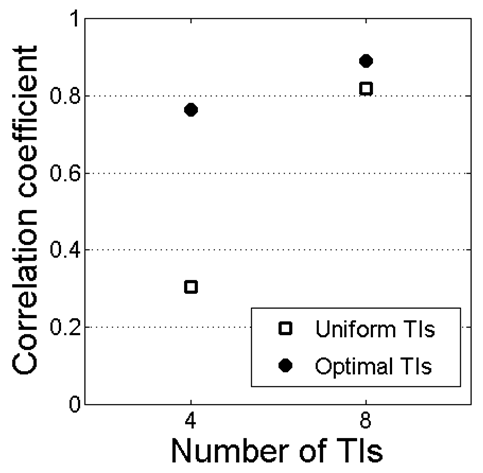
Table 1 lists the TIs used for each downsampling scheme and their expected $$$\overline{\xi}$$$ values computed from equation 3. ΔF from uniformly-sampled 4-TI data was 110±107mL/min/100g, significantly larger (P=0.03) than ΔF from optimally-sampled 4-TI data: 66±59mL/min/100g (Figure 2). With 8 TIs, the difference in ΔF between uniform sampling (62±54mL/min/100g) and optimal sampling (50±52mL/min/100g) was not significant (P=0.19). Correlation between reference and 4-TI perfusion estimates was higher with optimal sampling (R=0.76) than with uniform sampling (R=0.30). For 8 TIs, correlation with reference was R=0.82 with uniform sampling and R=0.89 with optimal sampling (Figure 3).Discussion
Optimization of TI selection with the proposed method significantly increased the precision and accuracy of renal perfusion estimates from ASL data sampled at few TIs. Because TI optimization allows for more reliable perfusion estimates from fewer TIs, it can reduce the scan time and number of breath-holds necessary for examining renal perfusion with ASL.Acknowledgements
References
1. Alsop DC, Detre JA, Golay X, et al. Recommended implementation of arterial spin-labeled perfusion MRI for clinical applications: A consensus of the ISMRM perfusion study group and the European consortium for ASL in dementia. Magn Reson Med 2015;73(1):102-116.
2. Conlin CC, Zhao Y, Zhang JL. Improving the accuracy of renal perfusion measurements from ASL by using multiple TIs: Validation with DCE MRI. Proc Int Soc Magn Reson Med 24 (2016).
3. Zhang JL, Sigmund EE, Rusinek H, et al. Optimization of b-value sampling for diffusion-weighted imaging of the kidney. Magn Reson Med 2012;67(1):89-97.
4. Zhang JL, Koh TS. On the selection of optimal flip angles for T1 mapping of breast tumors with dynamic contrast-enhanced magnetic resonance imaging. IEEE Trans Biomed Eng 2006;53(6):1209-1214.
Figures