Synopsis

Using feature-tracking combined with variable tag strength and flip angle, myocardial strain is measured and compared against traditional tagging MRI in healthy volunteers .

Purpose:

Myocardial strain from MRI has gained acceptance in clinical and research settings over the last 3 decades. Gradient-recalled echo (GRE) grid-tagging¹ has been well validated, both in phantoms and in vivo with comparison to sonomicrometry². Calculating strain directly from untagged cine SSFP images by tracking image features via non-rigid registration has recently been reported^3,4. Although good agreement can be found in myocardial whole-wall circumferential strain measurements between the untagged SSFP and tagged GRE, regional strains show statistically significant discrepancies⁵.

Here we aim to investigate the effects of different imaging parameters (tagging strength and imaging flip angle) on the measurement of myocardial strain using non-rigid registration methods. This was tested in healthy individuals using GRE tagging, untagged SSFP, and tagged SSFP (LISA-SSFP⁶).

Methods:

Scan setup: Fifteen healthy volunteers (34.9 ± 13.6 years old, 12 female) were imaged following informed consent using a clinical 3T MRI (Magnetom Skyra, Siemens Healthcare, Germany). All of the subsequent scans were performed in the same short-axis mid left ventricular slice for comparison.

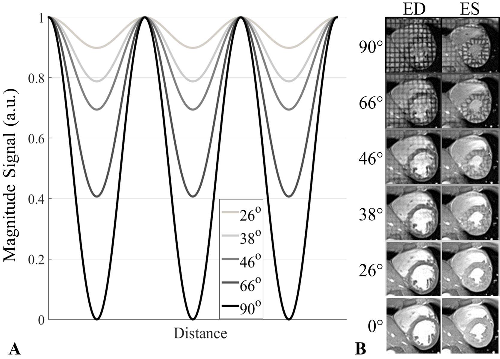
GRE Tagging RF dependency: The effect of tag strength can be explored using the tagged GRE technique. By ramping down the total binomial tagging radiofrequency angle (β), decreasing tagging strength is achieved. The effect of β on the magnitude of the tagging pattern can be modelled according to Fischer⁷ (see Figure 1A).

Here the standard GRE tagging sequence, which employs a binomial tagging structure, was modified in a prototype to ramp down the tagging strength, investigating 6 variations of β: 90° (full saturation), 66°, 46°, 38°, 26°, and 0° (no RF but tagging block still played out).

Typical imaging parameters were: FLASH imaging sequence, TR / TE = 5.62 / 2.66 ms, α = 12⁰, slice thickness = 6 mm, FOV = 320 x 262 mm², image matrix = 224 x 184, 1.43 x 1.43 mm² in-plane resolution, retrospective gating, 12 segments, 25 reconstructed cardiac timeframes, 8 mm grid spacing.

Imaging RF dependency in untagged SSFP: In untagged SSFP imaging at 3T, blood-myocardium contrast can be maximized based on tissue T1 and T2, occurring at approximately α = 50° for typical TR and TE and SAR limitations. To test the effect of lowering α on strain calculations in untagged SSFP images, 5 variations of α were used: 50°, 40°, 30°, 20°, and 10°. Imaging parameters were: TR / TE = 3.36 / 1.47 ms, slice thickness = 6 mm, FOV = 320 x 262 mm², image matrix = 224 x 184, 1.43 x 1.43 mm² in-plane resolution, iPAT = 2 (44 reference lines), retrospective gating, 12 segments, 25 reconstructed cardiac timeframes.

LISA-SSFP tagging parameter optimization: When considering SSFP tagging, tag persistence needs to be maintained to end-systole (ES) for accurate strain assessment. However, tags fade more quickly as α is increased, so that utilizing clinical values of α can be problematic. Previous work employing SSFP tagging has shown that an α of approximately 30-40° allows for persistence to ES (~400 ms) at 3T⁸. In this study we aimed to find the correct balance between α and β that gives clinically diagnostic SSFP contrast and accurate ES regional strain measures as compared with fully-saturated GRE tagging (here used as the ‘gold standard’); 12 combinations of α and β were implemented.

These images were acquired with a prototype version of LISA-SSFP tagging using 1-3-3-1 binomial tagging. Typical parameters were: TR / TE = 3.36 / 1.47 ms, slice thickness = 6 mm, FOV = 320 x 262 mm², image matrix = 224 x 184, 1.43 x 1.43 mm² in-plane resolution, iPAT = 2 (44 reference lines), retrospective gating, 12 segments, 25 reconstructed cardiac timeframes, 8 mm grid spacing.

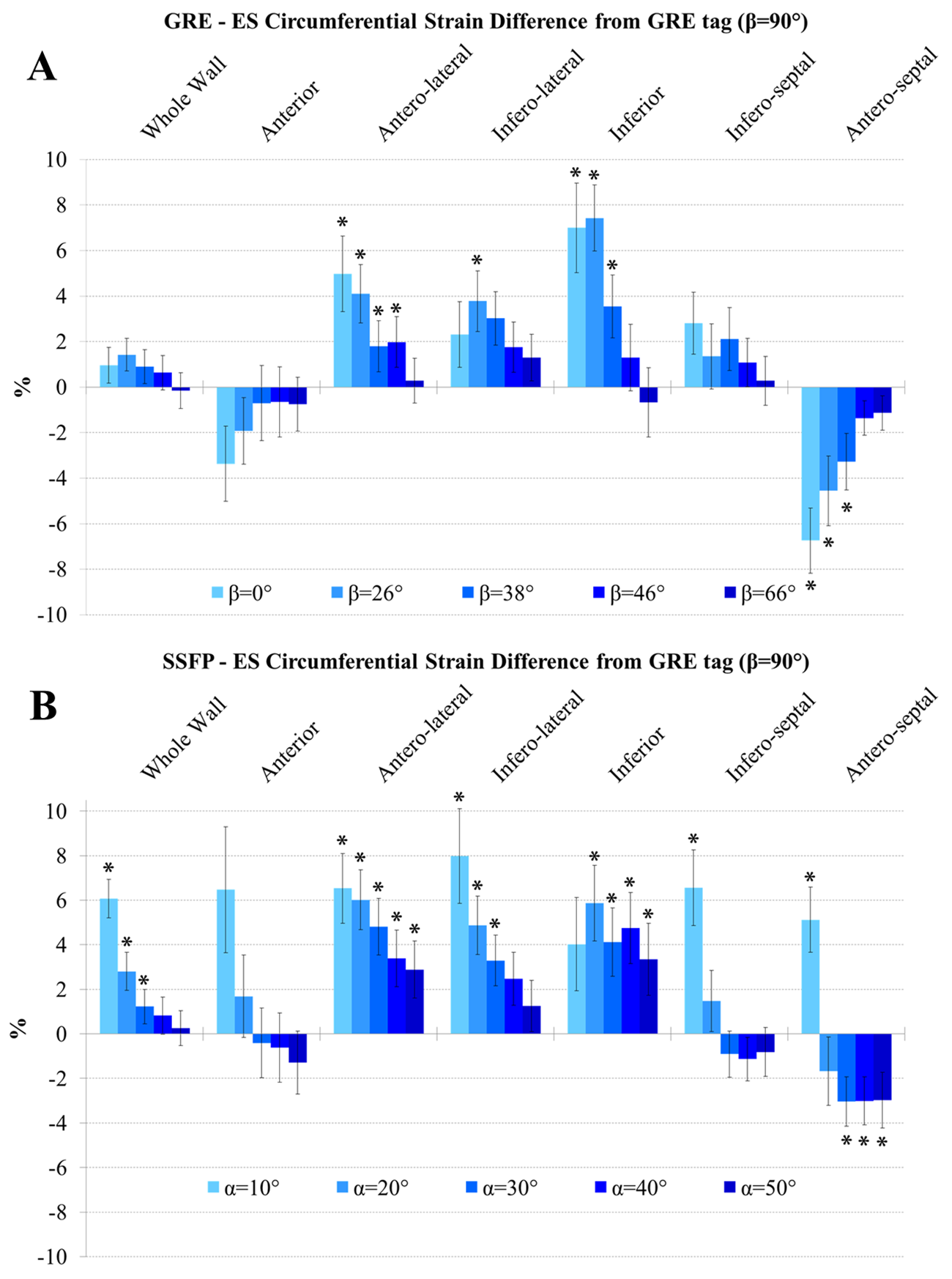
Analysis and statistics: All images were analysed using the Cardiac Imaging Modeller (CIM, University of Auckland, New Zealand). ES circumferential strain was assessed: averaged over the entire myocardial wall, and in 6 AHA segments according to anterior and posterior insertions of the right ventricle in the septum. GRE tagging using β = 90° (full saturation) was used as the ‘gold standard’, and differences across imaging parameter variations were calculated for comparison. Across regions, paired t-tests were performed with p < 0.05 considered statistically significant. Multiple comparisons were corrected using false discovery rate⁹.

Results:

Figure 1B demonstrates the ramping down of β in a healthy volunteer. At the lowest nonzero value of β = 26°, the tagging grid is slightly visible at end-diastole (ED).

Results for ES circumferential strain differences from the ‘gold standard’ GRE averaged (± standard error) over all volunteers across variations of β are shown in Figure 2A. At the lowest values of β, while whole wall strain is preserved, larger and statistically significant segmental differences are observed. As tagging magnitude is increased, regional differences become smaller. Figure 2B displays strain differences across flip angles in untagged SSFP. As α drops, whole wall differences become statistically significant.

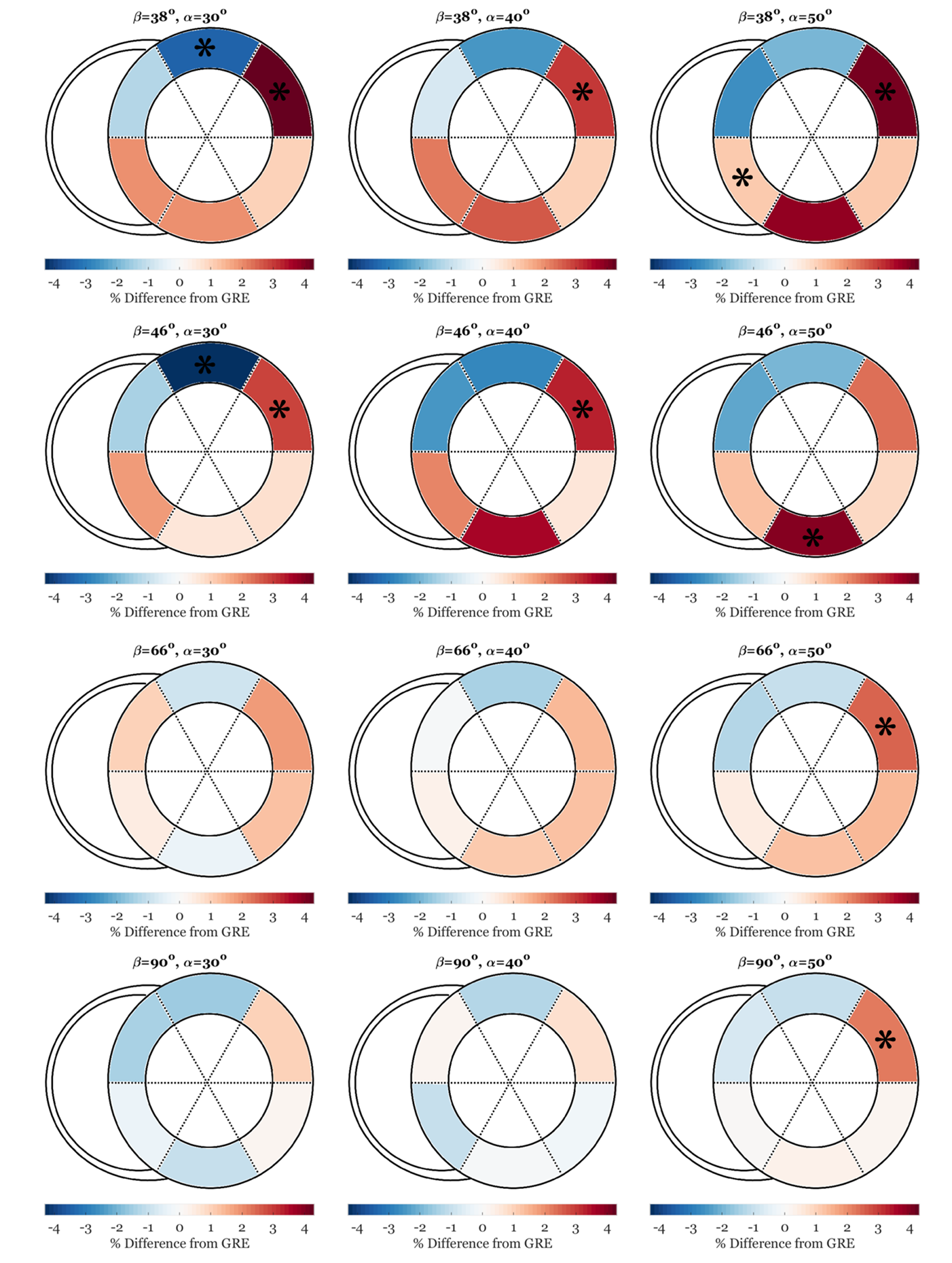
Short-axis graphical representation of strain differences across variations in α and β from SSFP tagging are shown in Figure 3. At high β, differences were statistically insignificant. At combinations of both lower α and lower β, differences were greater. Across all regions differences were less than 4%, and statistically significant differences only consistently appeared in the anterolateral region.

Conclusion:

This study quantified the dependence of myocardial circumferential ES strain measurements on imaging flip angle and tagging magnitude. In GRE tagging, lower tagging appears to give reasonable regional results, while a cutoff of α > 20° seems to give the best measurements in untagged SSFP. With visible tagging patterns, non-rigid registration tracking (and thus strain) is primarily determined by myocardial features; as these patterns fade or are reduced, extracardiac features begin to dominate the tracking algorithms. This in turn causes regional strain errors related to surrounding extracardiac structures.

The results in SSFP tagging display the potential to gain SSFP-like contrast (with α > 20°) with low-level tagging, all while maintaining regionally correct values of strain. This provides the framework for establishing a ‘subtly’ tagged SSFP acquisition that could be used to garner both ventricular volumetrics and myocardial strain within the same acquisition.

Acknowledgements

References

1. Axel L, Dougherty L. Heart wall motion: improved method of spatial modulation of magnetization for MR imaging. Radiology 1989; 172(2): 349-50.

2. Young AA, Axel L, Dougherty L, Bogen DK, Parenteau CS. Validation of tagging with MR imaging to estimate material deformation. Radiology 1993; 188(1): 101-8.

3. Li B, Young AA, Cowan BR. GPU accelerated non-rigid registration for the evaluation of cardiac function. Med Image Comput Comput Assist Interv 2008; 11(Pt 2): 880-7.

4. Augustine D, Lewandowski AJ, Lazdam M, Rai A, Francis J, Myerson S et al. Global and regional left ventricular myocardial deformation measures by magnetic resonance feature tracking in healthy volunteers: comparison with tagging and relevance of gender. J Cardiovasc Magn Reson 2013; 15: 8.

5. Cowan BR, Peereboom SM, Greiser A, Guehring J, Young AA. Image Feature Determinants of Global and Segmental Circumferential Ventricular Strain From Cine CMR. JACC Cardiovasc Imaging 2015; 8(12): 1465-6.

6. Zwanenburg JJ, Kuijer JP, Marcus JT, Heethaar RM. Steady-state free precession with myocardial tagging: CSPAMM in a single breathhold. Magn Reson Med 2003; 49(4): 722-30.

7. Fischer SE, McKinnon GC, Maier SE, Boesiger P. Improved myocardial tagging contrast. Magn Reson Med 1993; 30(2): 191-200.

8. Markl M, Reeder SB, Chan FP, Alley MT, Herfkens RJ, Pelc NJ. Steady-state free precession MR imaging: improved myocardial tag persistence and signal-to-noise ratio for analysis of myocardial motion. Radiology 2004; 230(3): 852-61.

9. Glickman ME, Rao SR, Schultz MR. False discovery rate control is a recommended alternative to Bonferroni-type adjustments in health studies. J Clin Epidemiol 2014; 67(8): 850-7.