Introduction

Myocardial T₁ mapping sequences enable quantitative assessment of diffuse myocardial fibrosis. In these sequences, a series of T₁-weighted (T₁-w) images are acquired and used for pixel-wise estimation of T₁ values by curve fitting. However, motion between these images often results in artifacts. The in-plane motion mostly appears as displacements of the myocardium in the image, while through-plane motion induces some scaling, combined with slight variations in myocardial shape. Therefore, motion correction is commonly used to correct for in-plane motion in myocardial T₁ mapping^1-3. In this work, we introduce a new non-rigid registration method based on modelling the image intensity at different ranges of inversion times along the relaxation T₁ to compensate for respiratory and cardiac motions.

Methods

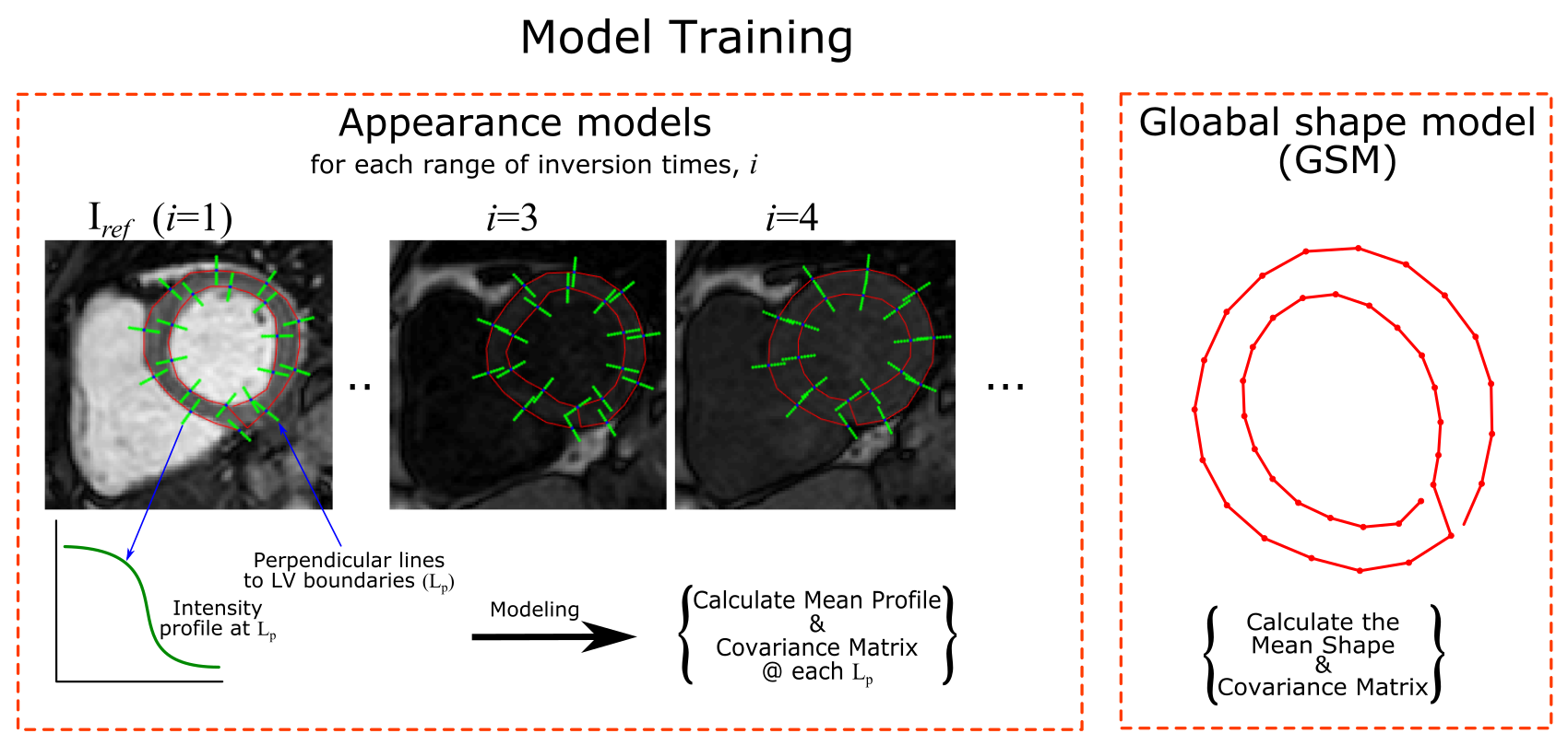
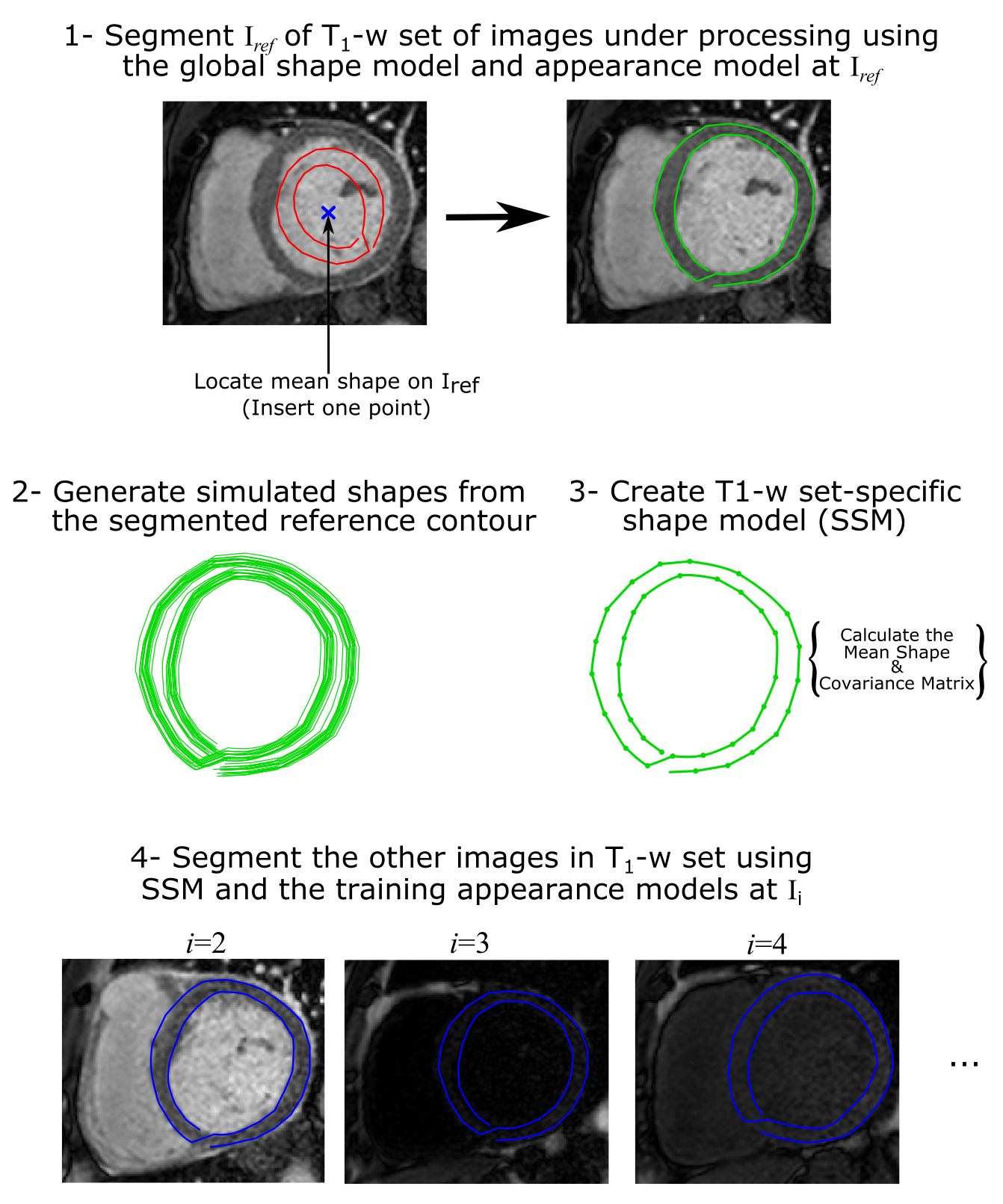
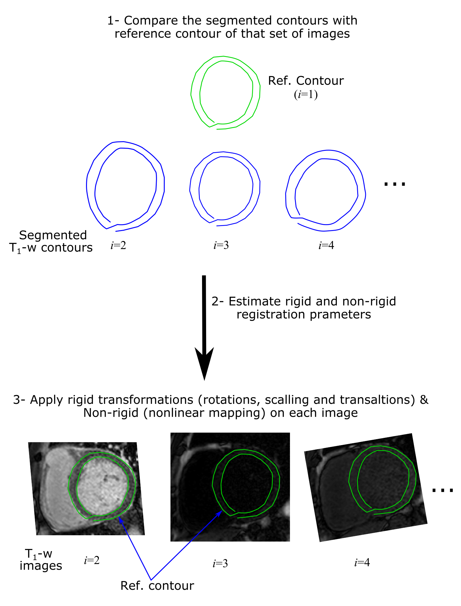
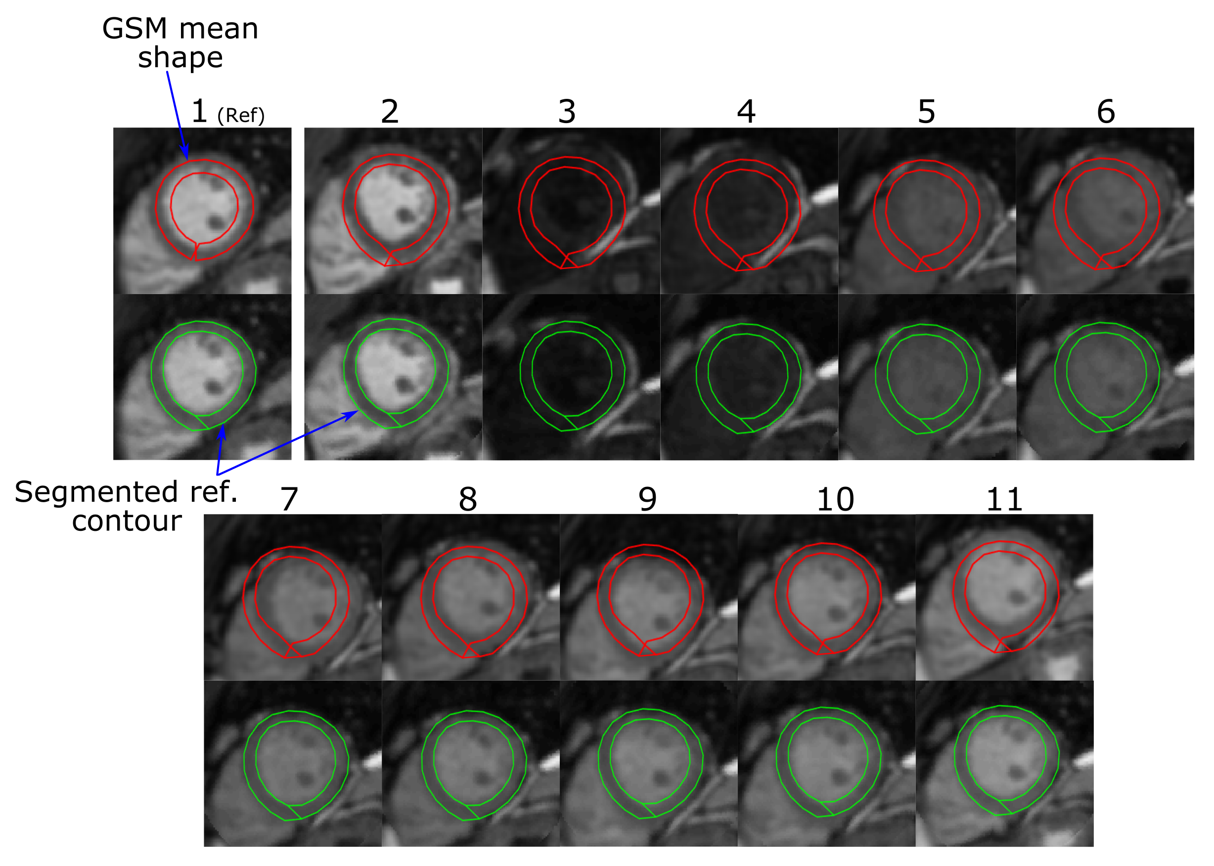
One of the challenging issues in motion correction in T₁ mapping is rapid variation of image contrast/intensity between different T₁-w images. We propose to use an Active Shape/appearance Model (ASM)-based framework to model the variations of the image intensity of Left Ventricular (LV) myocardial boundaries of different T₁-w images of T₁ mapping sequence (Fig. 1). To train this model, intensity profiles along the perpendicular lines to both epi- and endocardial boundaries are extracted at different spatial landmarks from different subjects in a training dataset. Mean and covariance matrices of the captured profiles are then calculated to represent the expected intensity at each range of inversion times, i, and its modes of variation. Another shape model (GSM), is built for LV myocardium where epicardium and endocardium boundaries are manually delineated. Then, the mean and covariance matrix of extracted contours are calculated. In segmentation, the mean shape of GSM model is inserted into the reference image, I_ref. In this work we chose to use the T₁-w image with highest contrast as reference. This initial mean shape is iteratively evolved using a matching algorithm to segment the myocardium, guided by the models built during training (Fig. 2). The final segmented contour (C_ref) of I_ref is used to generate a new shape model (SSM) specific to the T₁-w set of images, I_i; where i is the inversion time index. Simulated scaling factors and additive shifts, similar to those caused by respiratory motion, are generated from a Gaussian distribution and applied to C_ref to produce a number of simulated shapes specific to this set of T­­₁-w images. The SSM model is then used with the training appearance models at each inversion time to segment the other Ii images and generate set of corresponding contours, C_i. Rigid and non-rigid parameters between the two contours, C_ref and each C_i, are calculated and applied to the i^th image, I_i, using rigid transformations (rotation, scaling and translation), and nonlinear image warping (mapping) for the non-rigid parameters (Fig. 3). To evaluate the proposed algorithm, we have acquired myocardial T₁ maps in 60 patients with known or suspected cardiovascular disease. Imaging was performed using a 1.5T Philips Achieva system. Native T₁ mapping was performed using free-breathing slice-interleaved T₁ (STONE) sequence⁴ with the following parameters: TR/TE = 2.7/1.37 ms, FOV = 360×351 mm², acquisition matrix = 172×166, voxel size = 2.1×2.1 mm², slice thickness = 8 mm, and flip angle = 70^o. The dataset was divided into two equal parts: 30 patient-datasets for training and 30 patient-datasets for testing the model. For all cases, the LV epi- and endocardial boundaries were manually delineated and the extracted contours were considered as the ground truth for training and validating the model. The proposed framework is quantitatively validated by calculating Dice index and Hausdorff measure between the manual segmented contours and the contours produced after registration.

Results

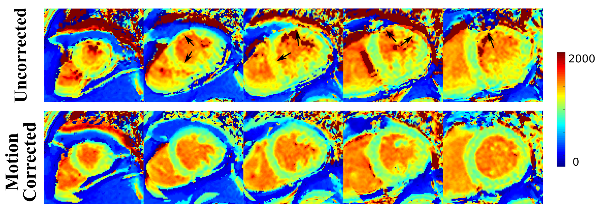
Figure 4 shows the T₁ maps at 5 short axial slices before and after registering the T₁ images. Motion correction removes the artifacts associated with motion between different T₁-w images. Figure 5 shows an example of registering a set of T₁-w images, as well as the automatic segmentation of I_ref. All T₁-w images showed good mapping for both myocardium and blood after applying the registration parameters. Dice similarity index was increased from 0.901±0.09 before correction to 0.93±0.06 after using the proposed method (p<0.05). The average Hausdorff measure was decreased from 7.1±5.4 mm to 5.6±4.4 before and after the correction, respectively, (p<0.05). The computation time for training the framework was ~90 s, and that for registering a T₁-w set of 11 image was ~5 s with two image resolutions using a Matlab implementation on intel Xenon, 2.8 Hz CPU.

Conclusion

The proposed framework for registering T₁ weighted images based on ASM improves image quality of T₁ maps by minimizing the impact of motion.

Acknowledgements

No acknowledgement found.