Synopsis

The aim of the present work is to address the challenge of optimal flip angle calibration of ¹³C surface coils in hyperpolarization studies. To this end, we characterize the spatial profile of the flip angle and demonstrate that it allows for a simple calibration improving the signal-to-noise ratio for hyperpolarized ¹³C magnetic resonance spectroscopic imaging.

Introduction

For hyperpolarized ¹³C magnetic resonance spectroscopic imaging (¹³C-MRSI), flip angle (FA) calibration is challenged. Therefore, a ¹³C enriched phantom placed outside the imaged object is commonly used as reference. This does, however, give potential errors in case of RF transmit field (B₁) inhomogeneities directly affecting the FA. The common use of single-channel surface coils with strong RF transmit profiles for ¹³C-MRSI enhances the importance of addressing FA calibration.

The aim is to address optimal FA calibration of ¹³C surface coils. We characterize the spatial profile of the FA and demonstrate that it allows for a simple calibration improving the SNR.

Methods

Theory: The B₁ profile in the axial-axis of a surface loop coil is given by the Biot-Savart law. The coil transmitter voltage $$$V$$$ required for constant FA as function of distance is:

$$V(z)=c\cdot\left(z^2+a^2\right)^{3/2}\quad\quad\text{(1)}$$

where $$$c$$$ is an acquisition- and coil-dependent constant, $$$z$$$ is the axial-axis distance, and $$$a$$$ is the radius of the coil loop.

From Eq. (1) the following expression can be stated:

$$V_{90}(z)=V_{90,REF}\cdot\left(\frac{z^2+a^2}{z^2_{REF}+a^2}\right)^{3/2}\quad\quad\text{(2)}$$

Using Eq. (2), with a 90° FA calibrated at a reference position through determination of $$$V_{90,REF}$$$, a calibration $$$V_{90}(z)$$$ can hereby be obtained at an arbitrary position $$$z$$$ on the axial-axis.

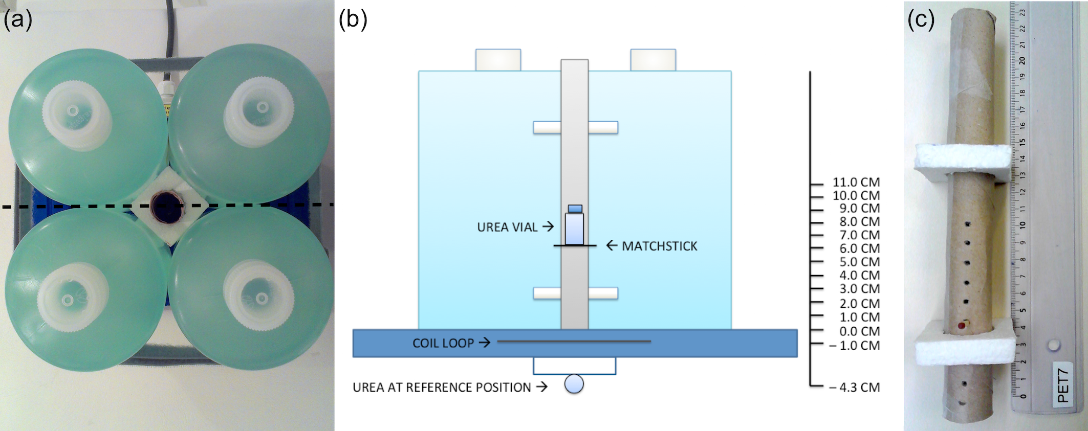
Phantom experiments: To verify Eq. (2) the FA profile was characterized for three different RF surface coils using the phantom setup in Figure 1.

The coils were: 1) a dual-tuned, ¹H/¹³C, transmit/receive 11 cm flex coil, 2) a ¹³C, transmit/receive 12 cm loop coil, and 3) a ¹³C, transmit/receive 20 cm loop coil (RAPID Biomedical). A 5.5 mL vial of 4.0 M ¹³C-urea was used for FA calibration. All scans were performed on the integrated 3T PET/MRI system (Siemens Biograph mMR).

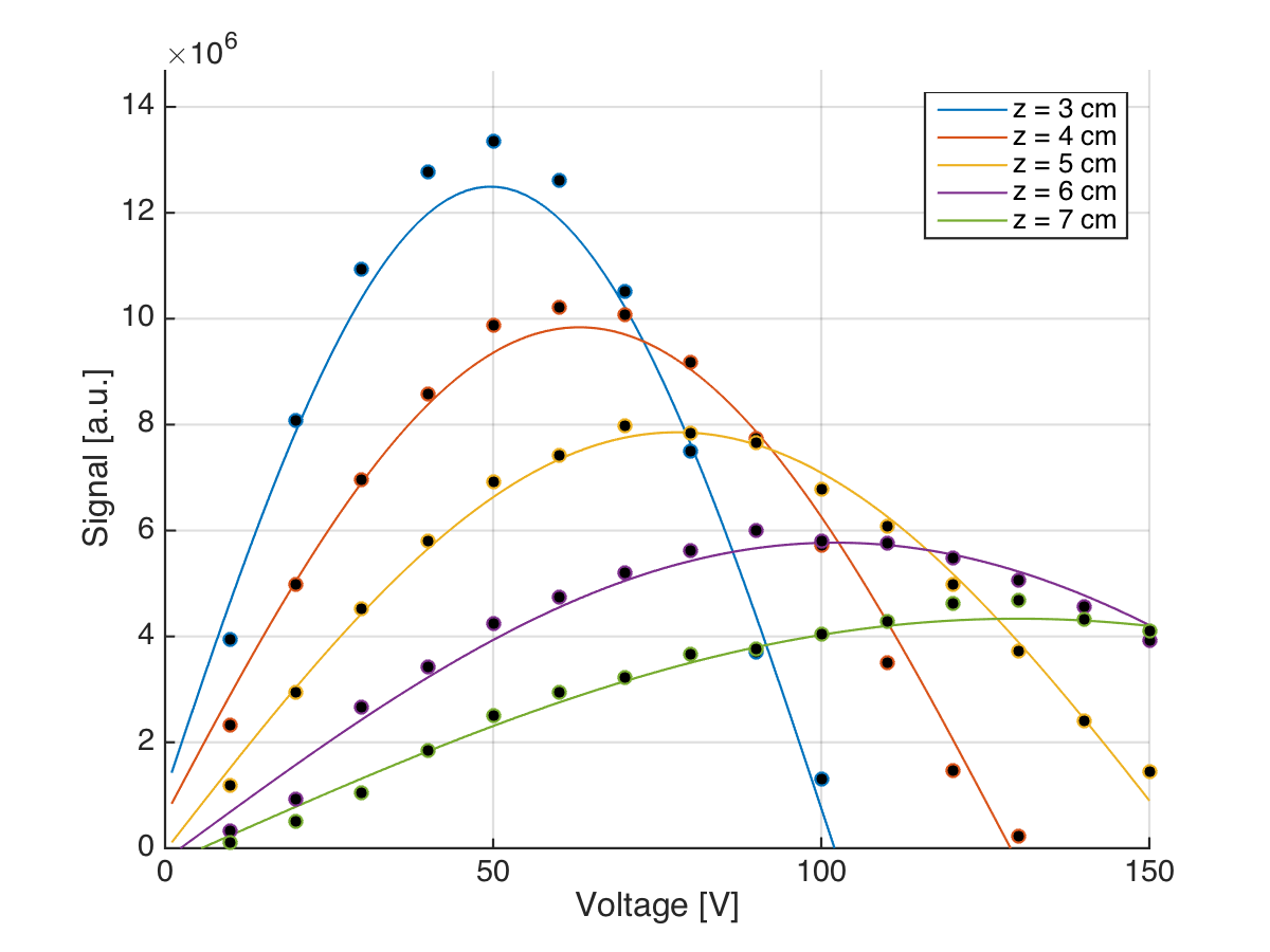
The vial was placed at a new position for each scan session, consisting of a localizer followed by FA calibration. For calibration a series of FID measurements with increasing transmitter voltage (10 V steps) were acquired [TR/TE 10,000/0.35 ms, FA 90°, BW 3,000 Hz, transmitter voltage 10 to 300 V (loop coils), transmitter voltage 10 to 150 V (flex coil)]. Spectra were centered on ¹³C-urea. A sinusoidal fit of the ¹³C-urea peak versus transmitter voltage was used to determine $$$V_{90}$$$. Eq. (1) was fitted to the calibration $$$V_{90}$$$ versus position of the ¹³C-urea vial. Experiments were repeated at different days and with different coil loads.

In vivo experiment: The feasibility of the calibration method was demonstrated in a canine cancer patient (39 kg) with a biopsy-verified axillar soft tissue sarcoma scanned as part of clinical staging work up. Patient handling and acquisition details are given in Gutte et al. 2015¹.

Hyperpolarized ¹³C-CSI was acquired with $$$V_{90,REF}=87.4$$$ V as measured using the calibration phantom positioned at the coil surface (equivalent to 90° at 2.3 cm). The CSI slice (13 mm slice thickness) was aligned parallel to the flex coil at a depth of 4 cm. To compensate for the FA loss a second CSI was obtained with $$$V_{90}=136$$$ V calculated by means of Eq. (2).

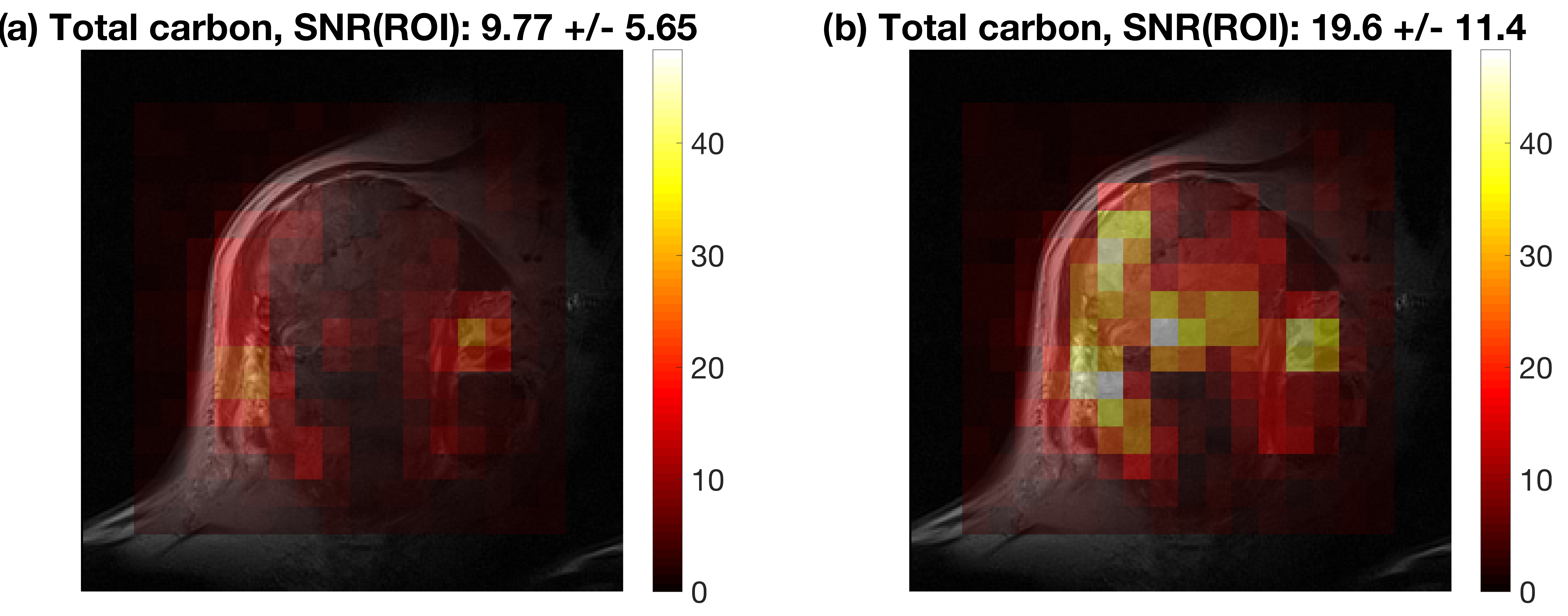
Voxel-wise SNR was estimated as the total carbon signal (sum of absolute peak values for pyruvate, pyruvate-hydrate, lactate, alanine, and bicarbonate) divided by five times the spectral noise (standard deviation of the real spectrum in noise regions).

Results

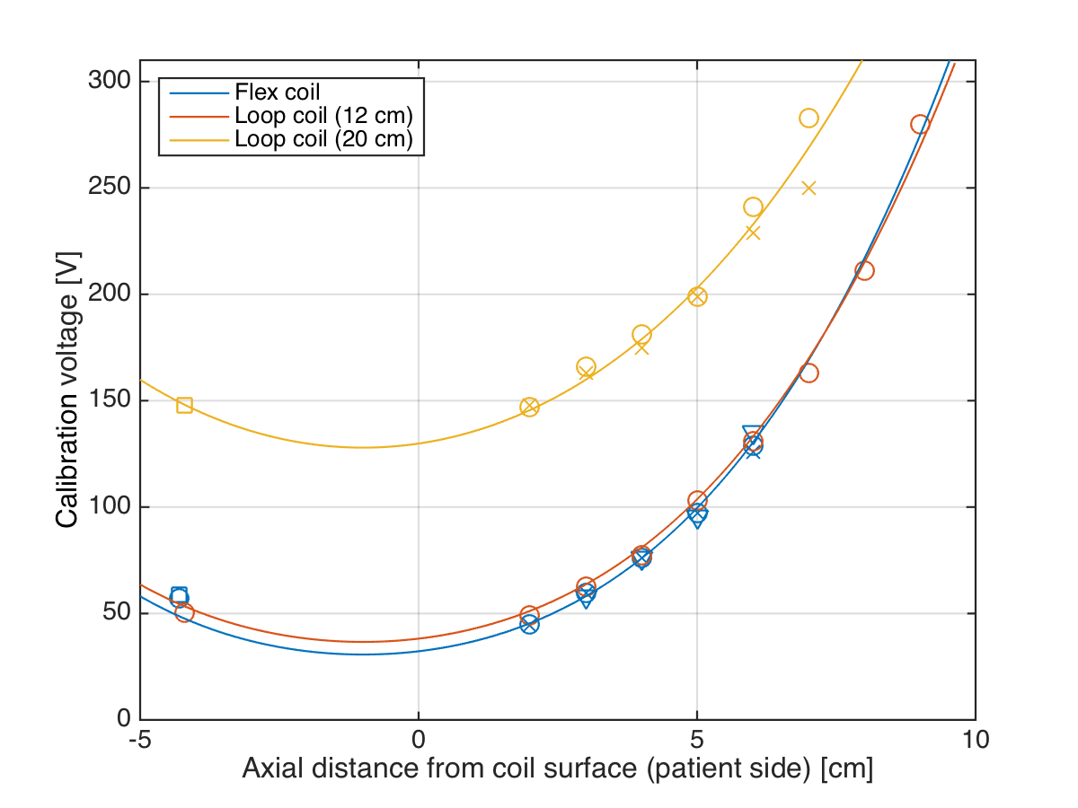
Figure 2 shows an example of FA calibration measurements and sinusoidal fits at different positions of the urea vial. The resulting calibration voltage $$$V_{90}$$$ and fits to Eq. (2) are shown in Figure 3. The fitting coefficients were: flex coil, $$$c=0.1847$$$ V/cm³ ($$$r^2=0.9807$$$); loop coil (12 cm), $$$c=0.1697$$$ V/cm³ ($$$r^2=0.9959$$$); loop coil (20 cm), $$$c=0.1280$$$ V/cm³ ($$$r^2=0.9681$$$). As can be appreciated in Figure 3 and by the $$$r^2$$$-values, data obtained for different days and loads follow the same curve.

Figure 4 shows SNR for the two ¹³C-MRSI scans of the soft tissue sarcoma. The SNR improvement factor was 2.01. The noise level was constant.

Discussion

Conclusion

Acknowledgements

References