2999
Absolute Quantification of Brain Metabolites at 3T: Methods and Pitfalls1Department of Neurobiology and Behavior, University of California, UCI, Irvine, CA, United States, 2Department of Neurology, University of California, UCI, Irvine, CA, United States, 3Center for the Neurobiology of Learning and Memory, University of California, Irvine, CA, United States
Synopsis
There exist several partial volume correction methods in the literature that often produce similar results. However, various tissue fractions can lead to substantial differences in estimated concentrations. These deviations are greater at longer TEs and greater cerebrospinal fluid contributions. In instances with a 75% WM fraction and no gray matter, the deviations can be up to 37% for TE of 135 ms at 3.0 T. These corrections were then applied to common regions of interest (ROI) in an MRS study involving 5 participants at 3T. By understanding where these methods deviate one can better make cross study comparisons.
Purpose
The purpose of this study was to compare several theoretical models of absolute metabolite quantification incorporating partial volume correction (PVC), and to determine instances in which these methods deviate from each other. These corrections were subsequently applied to three common regions of interest in an MRS study involving five healthy participants at 3T.Background
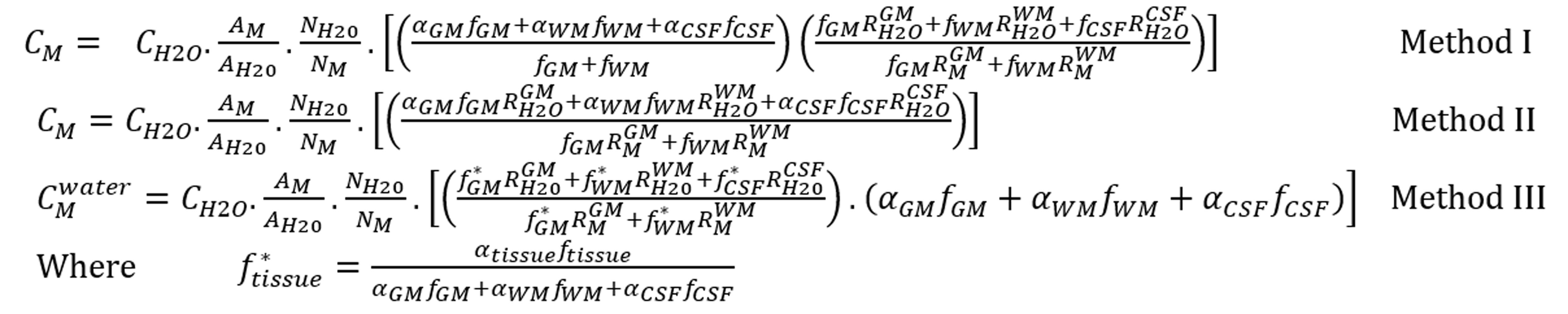
Quantitative MRS is achieved by comparing the water suppressed to water unsupressed spectra. Partial volume corrections account for the relative contributions of this signal originating from grey matter (GM) white matter (WM) and cerebrospinal fluid (CSF). By using a subject’s anatomical image, relative tissue fractions can be measured within the MRS voxel, and the variations in proton density and relaxation rates (T1, T2) between these tissues can be accounted for. We investigate three published methods for partial volume correction, shown in Figure 1. Method III has been modified from its original for to account for WM and GM relaxation separately rather than as an average. Method II has also been converted to units of mmol/L rather than mmol/kg wet weight.
Methods
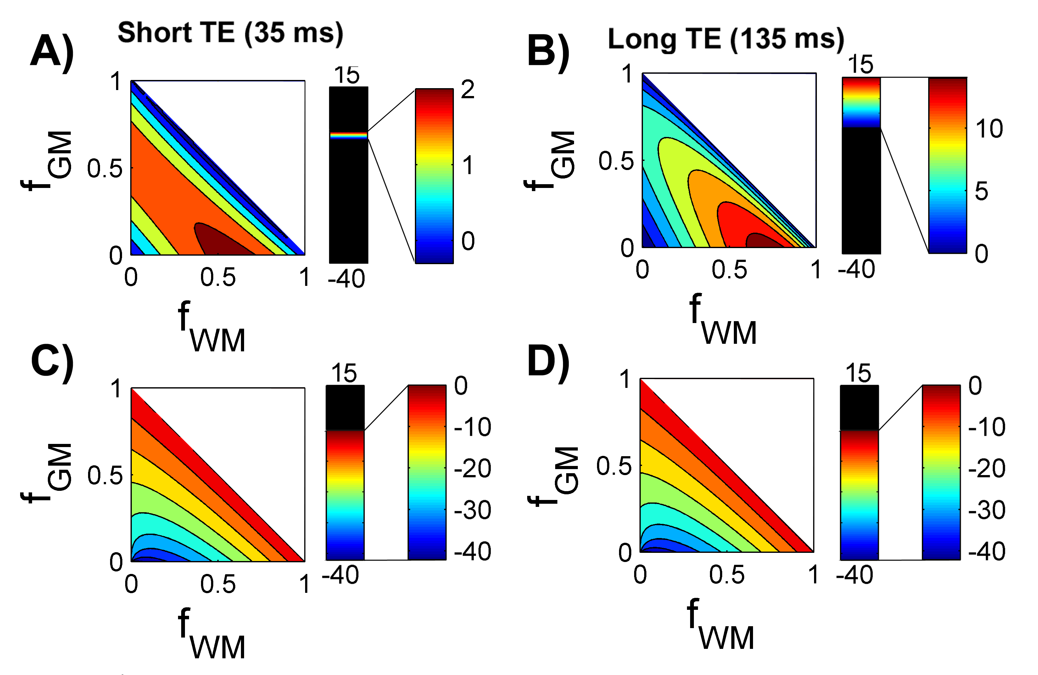
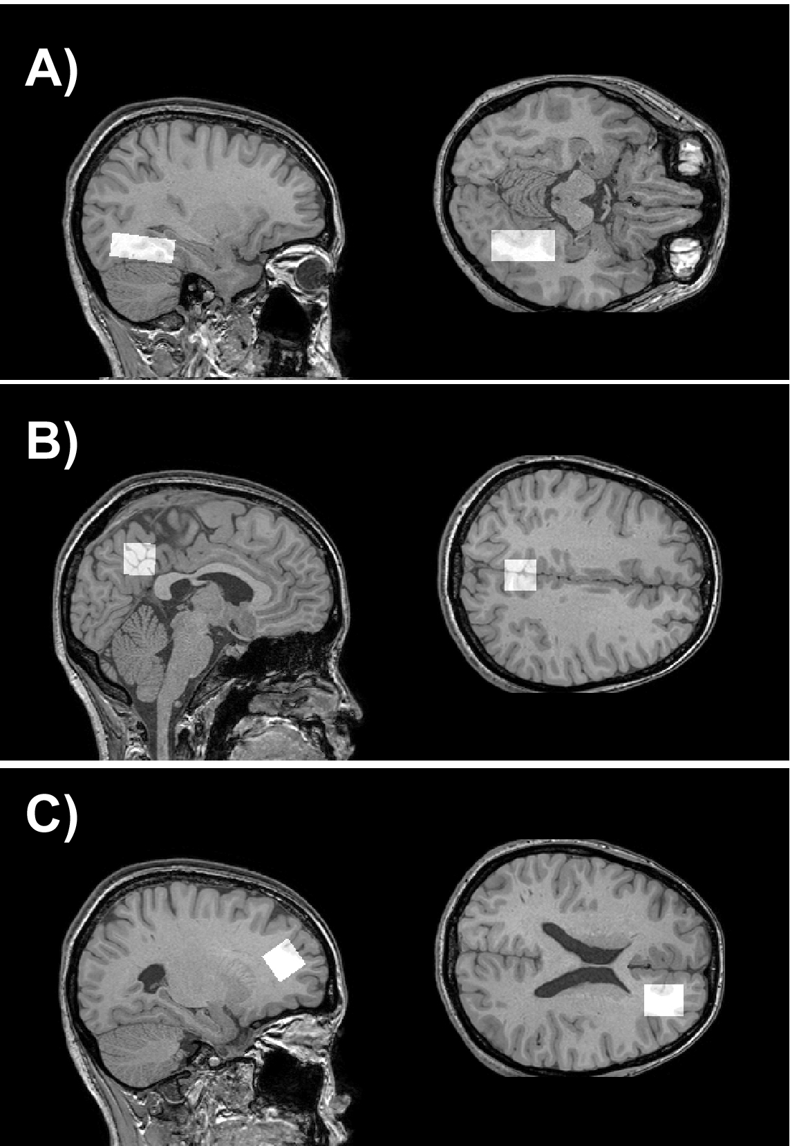
To determine the similarities (and differences) of the methods, all possible tissue fraction combinations were explored in simulations using MATLAB (the Mathworks, INC. Natick, MA). Each PVC method required an estimate for the percent water content (α) in each tissue and these values were one source of variance. Each method reported and used different constants in the calculations: (αGM=75%, αWM=65%,αCSF=100%) in the work of Gussew et al.[2]. Rupisingh et al.[1] and Bartha et al.[4] used: αWM=81%, αGM=71%,αCSF=100% and Ernst et al.[5] used αWM=78%, αGM= 65%, αCSF=97%. For a better comparison, a single water content fraction was used [2] for all calculations. The concentrations were corrected for water and metabolite T1 and T2 relaxation time constants using values for WM and GM obtained at 3T in healthy subjects [6]. Method II was used for comparisons between methods in Figure 2. The percent difference between pairs of methods (II-I and II-III) was defined as the difference divided by the pairwise mean and was calculated for all metabolites at both long (135 ms) and short (35 ms) TEs with a TR of 2000 ms. The percent difference reported was the average across all metabolites. To map these differences, each combination of tissue fraction was plotted such that fGM+fWM+fCSF=1. Data acquisition was done on a 3T Philips whole body MRI (Best, the Netherlands). Preliminary results are presented from five healthy volunteers. Spectra were acquired using a 2 x 2 x 2 cm3 single voxel PRESS sequence in the frontal and posterior cingulate areas and from a 4 x 2 x 1.5 cm3 voxel in the left parahippocampal cortex (TE=35 ms, 2048 data points).Results and Discussion
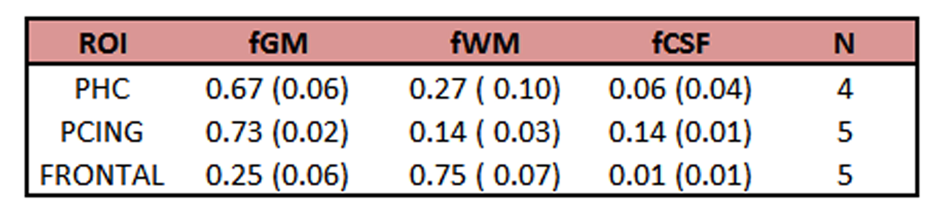
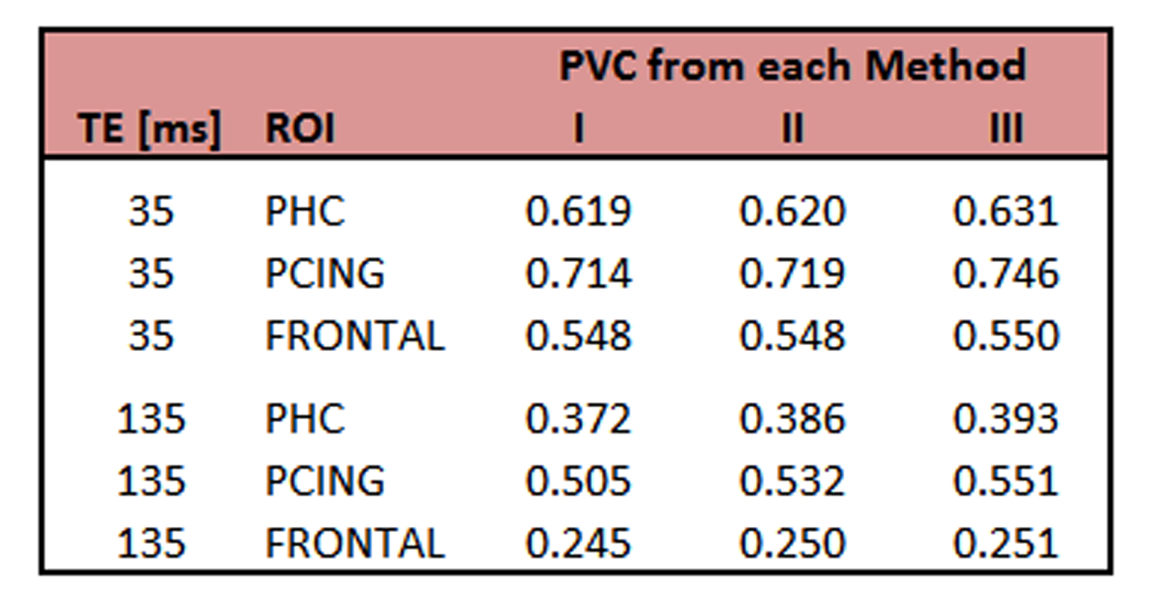
Figure 2 shows comparisons of all three methods for all possible combinations of tissue fractions at short and long echo times. All methods deviate with larger CSF contributions. From a theory perspective this is to be anticipated since the CSF term is introduced differently in each. For each comparison, the maximum deviation occurred at fGM=0%, but the fWM value varied. The percent difference between Methods II and I for short TE (Fig. 2A) was 2% and occurred at fWM=60%. For the long TE (Fig. 2B), the maximum difference was 15% (at fWM=75%). Method III deviated from Method II more substantially and followed a different pattern, peaking at -42% as fWM approached 0 (the areas with large proportion of CSF). Figure 3 shows the locations of all the commonly used ROIs in the frontal, posterior cingulate and parahippocampal areas of the brain. The corresponding corrections for each ROI are shown in Table 2. The practical results from five healthy volunteers at 3T are listed in Tables 1 and 2. There is negligible effect of choice of PVC method for ROIs with high GM content. The relatively large contributions of CSF in the posterior cingulate led to a 10% difference between methods long TE and 6% for short TE. The utility of quantitative MRS is to be able to compare absolute concentrations between field strengths and studies.
The possibility of PVC systematically modifying the concentration correction is a real concern. The similarities of these three methods (in certain instances) can mislead one into a false sense of confidence for the reliability and cohesiveness of methodologies for PVC in the field of MRS. By understanding where these methods deviate one can better compare between methods or even calculate appropriate scaling factors for retrospective meta-analysis. In general, these deviations are more pronounced for less GM, more CSF and longer TE.
Acknowledgements
No acknowledgement found.References
[1] R. Rupsingh, M. Borrie, M. Smith, J. L. Wells, and R. Bartha, “Reduced hippocampal glutamate in Alzheimer disease,” Neurobiol. Aging, vol. 32, no. 5, pp. 802–810, May 2011. [2] A. Gussew, M. Erdtel, P. Hiepe, R. Rzanny, and J. R. Reichenbach, “Absolute quantitation of brain metabolites with respect to heterogeneous tissue compositions in (1)H-MR spectroscopic volumes,” Magma N. Y. N, vol. 25, no. 5, pp. 321–333, Oct. 2012. [3] C. Gasparovic, T. Song, D. Devier, H. J. Bockholt, A. Caprihan, P. G. Mullins, S. Posse, R. E. Jung, and L. A. Morrison, “Use of tissue water as a concentration reference for proton spectroscopic imaging,” Magn. Reson. Med., vol. 55, no. 6, pp. 1219–1226, Jun. 2006. [4] R. Bartha, M. Smith, R. Rupsingh, J. Rylett, J. L. Wells, and M. J. Borrie, “High field (1)H MRS of the hippocampus after donepezil treatment in Alzheimer disease.,” Prog Neuropsychopharmacol Biol Psychiatry, vol. 32, pp. 786–93, Apr. 2008. [5] T. Ernst, R. Kreis, and B. Ross, “Absolute quantitation of water and metabolites in the human brain. 1: Compartments and water.,” J Magn Res Ser B, vol. 102, pp. 1–8, 1993. [6] G. J. Stanisz, E. E. Odrobina, J. Pun, M. Escaravage, S. J. Graham, M. J. Bronskill, and R. M. Henkelman, “T1, T2 relaxation and magnetization transfer in tissue at 3T,” Magn. Reson. Med., vol. 54, no. 3, pp. 507–512, Sep. 2005.Figures