2851

Image-based Background Phase Error Correction in 4D Flow MRI

Julia Busch¹, Daniel Giese², and Sebastian Kozerke^1,3

¹Institute for Biomedical Engineering, University and ETH Zurich, Zurich, Switzerland, ²Department of Radiology, University Hospital Cologne, ³Division of Imaging Science and Biomedical Engineering, King’s College London

Synopsis

Background phase errors occurring in 4D Flow MRI are analyzed with respect to their spatial order. Results demonstrate that background errors can range from first up to third spatial order requiring correction with appropriate polynomial orders. While higher order corrections perform well even for low SNR, they are highly sensitive to the amount of stationary tissue present for background phase estimation requiring at least 25%, 60% and 75% of stationary tissue for systems with first, second and third order offsets The amount of stationary tissue available in-vivo, however, limits the use of higher order polynomial models for background phase correction.

Purpose

4D Flow MRI is of increasing interest and use for various applications^1,2. To correct for residual background phase errors, image-based correction approaches by referencing through stationary tissue are widely used in practice^3-5. It is the aim of the present study to analyze background phase errors occurring in 4D Flow MRI.

Material and Methods

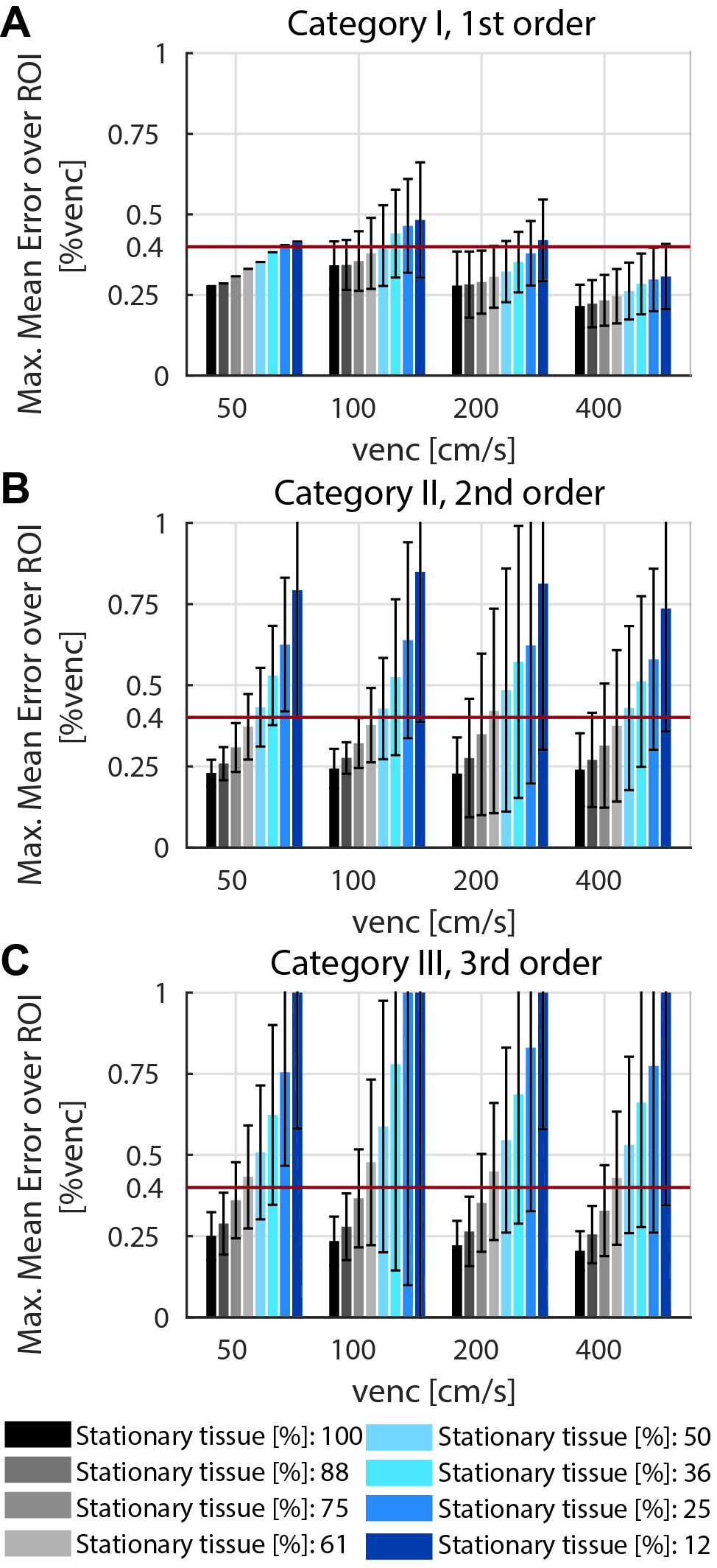
4D Flow MRI data was acquired for typical geometries and encoding velocities in a stationary phantom on two clinical Philips MR systems. Sequence parameters were chosen according to recommendations of the 4D Flow MRI consensus statement⁶. Background errors were analyzed with respect to their spatial order. Minimum requirements regarding the signal-to-noise ratio (SNR) and the amount of stationary tissue necessary for phase error estimation were assessed. On the phantom data, limited amount of stationary tissue for linear regression was simulated by assigning an elliptical volume of varying size in the center of the phantom data as non-stationary, thereby leaving the rim of the phantom as "stationary tissue".

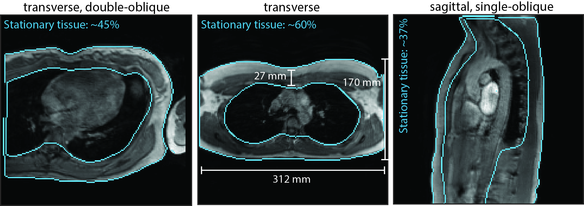
For comparison, volumes and locations of stationary tissue were derived from in-vivo data. Additionally for in-vivo validation, 4D Flow data of the aorta was acquired in 5 healthy subjects on one MR system including subsequent scans on the stationary phantom.

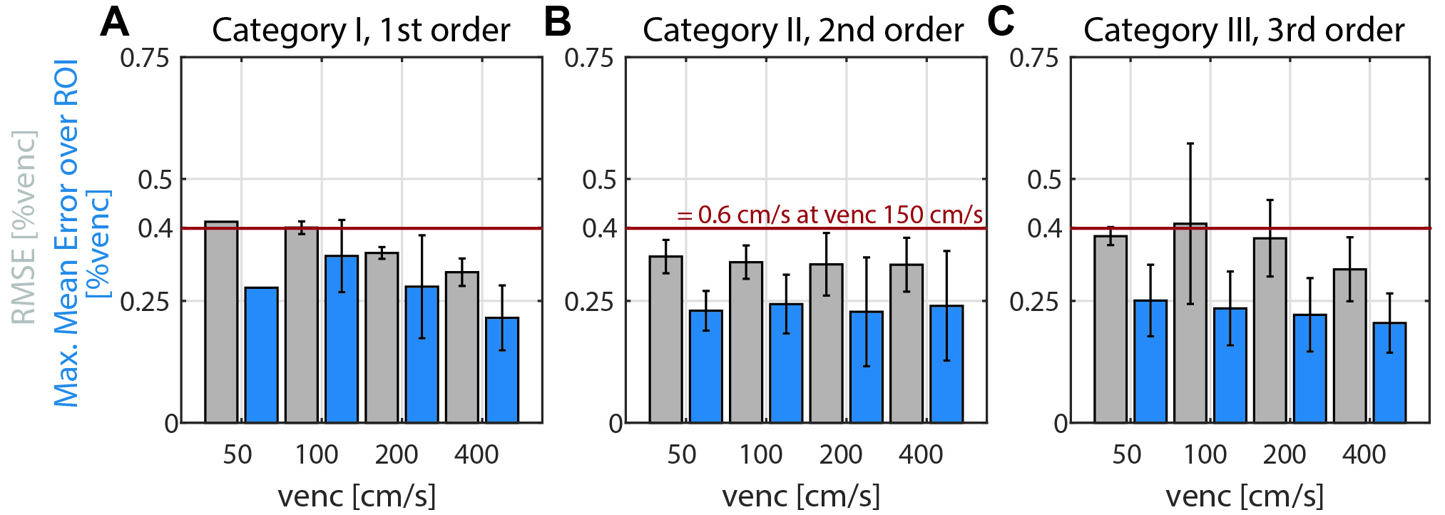
To assess the quality of linear regression the root-mean-square error (RMSE) was used. The RMSE is stated in % of the encoding velocity (%venc) and was calculated over the full imaged object volume. In addition, for the phantom study the mean error over all possible cubic regions-of-interest (ROIs) of 30x30x30mm³ was calculated and the maximum extracted: $$\max M{{E}_{ROI}}=\underset{ROIs}{\mathop{\max}}\,\left(\left|\frac{\sum\nolimits_{i\in ROI}{\left({{v}_{i}}-{{{\tilde{v}}}_{i}}\right)}}{{{N}_{ROI}}} \right|\right)$$

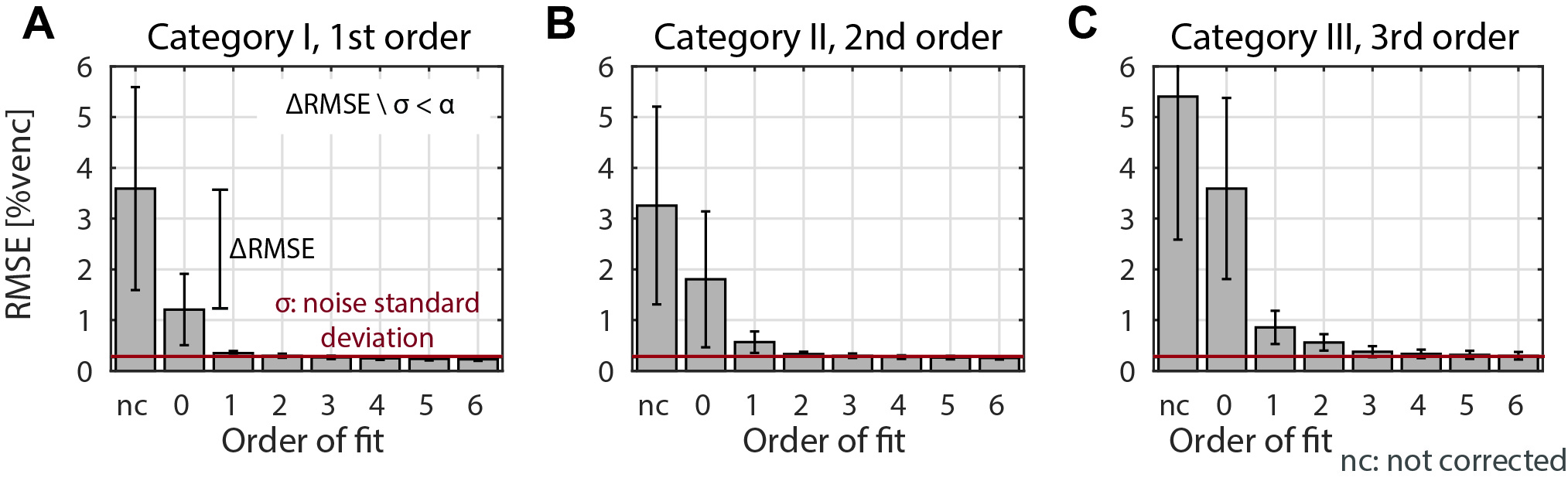
where $$$v_{i}$$$ is the measured data and $$${{\tilde{v}}_{i}}$$$ the estimated background phase at voxel $$$i$$$. The edge length of the ROIs was chosen to be 30mm in accordance to a typical aortic diameter. The maxME_ROI was evaluated over the inner 50% of the imaged object volume excluding regions which would be stationary in-vivo. A threshold of the maxME_ROI of 0.4 %venc was defined which would translate into an error of 0.6 cm/s for an encoding velocity of 150 cm/s which in turn corresponds to 5% error in stroke volume as a limit of acceptability⁷ for clinical applications. For in-vivo validation, particle trace counts at three locations in the aorta were computed. To analyze the spatial variation of the background error, the relative improvement in RMSE between consecutive spatial orders was analyzed and a threshold was set at 30% of the noise level defined as the RMSE after a sixth order correction.

Results

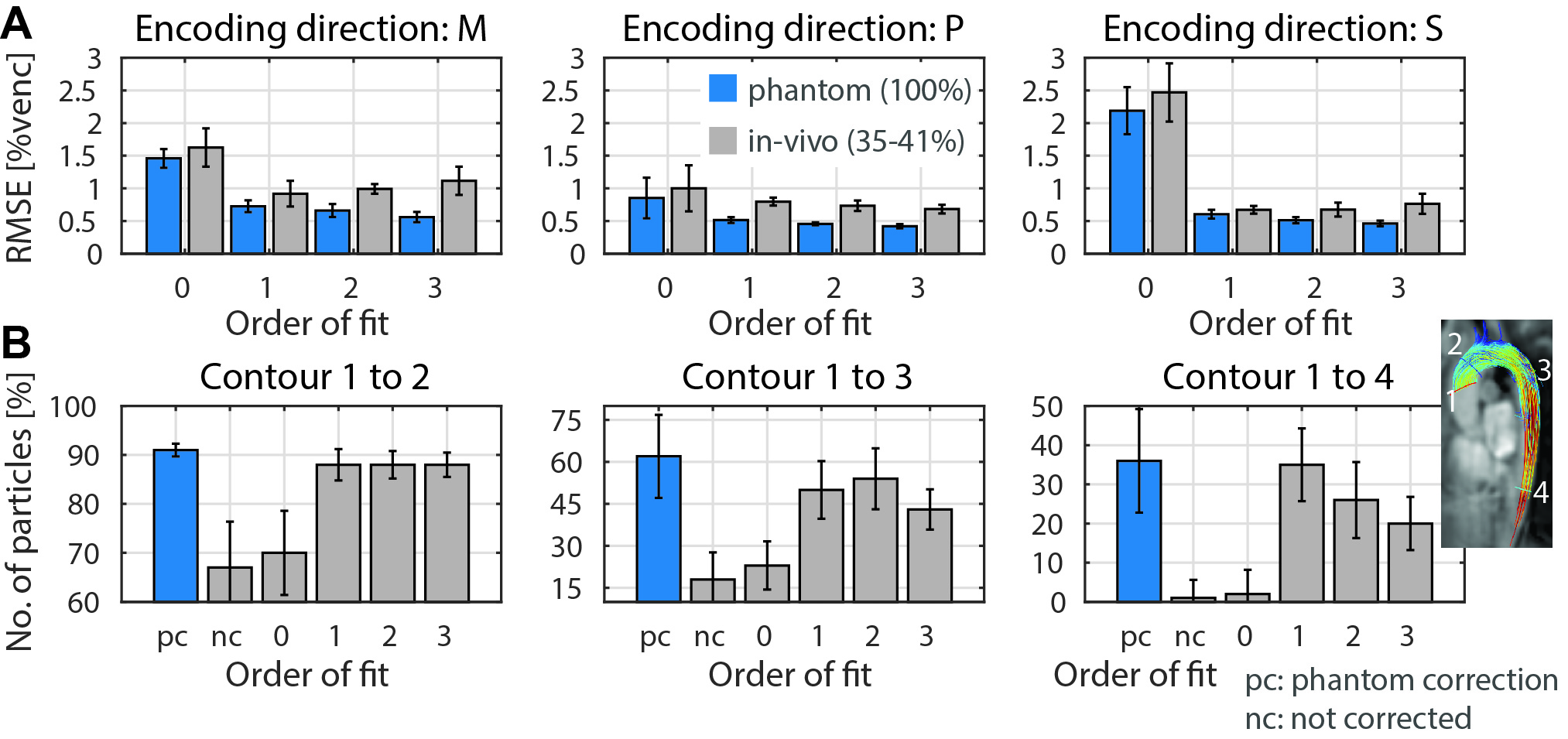
On the two MR systems used and for the different settings, spatial variation of background errors up to third spatial order were measured (Figure 1) and data was grouped into according categories, i.e. data in category I shows spatial variation of the background error up to first order. The maxME_ROI was below 0.4 %venc for all encoding velocities upon first, second and third order correction for category I, II and III, respectively (Figure 2). The residual error did not change significantly down to an SNR of 15 independently of the spatial order. The minimum amount of stationary tissue, however, was strongly dependent on the spatial order requiring at least 25%, 60% and 75% of stationary tissue for systems with first, second and third order offsets (Figure 3). In the volunteers measured, however, the amount of stationary tissue ranged from 35 to 63% of the total object volume depending on the geometry with an SNR ranging from 20 to 50 (Figure 4). The in-vivo validation of the aorta showed that with approximately 35-40% of stationary tissue available only first order correction yields a significant reduction in background phase error as exemplified by increased particle trace counts (Figure 5). Nonetheless, first order correction resulted in increased errors and reduced particle tracking accuracy when compared to the phantom correction using a third order polynomial model for estimation of the background offsets (Figure 5).

Discussion

Background phase errors can range from first to third spatial order requiring correction with appropriate polynomial orders. It is therefore recommended to test and adapt the order of background phase error correction for each individual MR system type and, accordingly, implement lower limits of the SNR and amount of stationary tissue depending on the polynomial order required for background phase correction. At the same time, however, the limited amount of stationary tissue typically available in-vivo limits image-based background phase error correction to zeroths and first spatial order despite the presence of higher order background phase errors. To this end, alternative correction methods including magnetic field monitoring^8-10 need to be studied further.

Acknowledgements

The authors thank Martin Bührer for support with the MRecon software package and acknowledge funding from the Swiss National Science Foundation, grant 320030_149567.

References

1. Markl M, Frydrychowicz A, Kozerke S, Hope M, Wieben O: 4D flow MRI. J Magn Reson Imaging 2012, 36:1015–36.

2. Srichai MB, Lim RP, Wong S, Lee VS: Cardiovascular Applications of Phase-Contrast MRI. Am J Roentgenol 2009, 192:662–675.

3. Caprihan A, Altobelli S, Benitez-Read E: Flow-velocity imaging from linear regression of phase images with techniques for reducing eddy-current effects. J Magn Reson 1990, 90:71–89.

4. Walker PG, Cranney GB, Scheidegger MB, Waseleski G, Pohost GM, Yoganathan AP: Semiautomated method for noise reduction and background phase error correction in MR phase velocity data. J Magn Reson Imaging 1993, 3:521–30.

5. Lankhaar J-W, Hofman MBM, Marcus JT, Zwanenburg JJM, Faes TJC, Vonk-Noordegraaf A: Correction of phase offset errors in main pulmonary artery flow quantification. J Magn Reson Imaging 2005, 22:73–9.

6. Dyverfeldt P, Bissell M, Barker AJ, Bolger AF, Carlhäll C-J, Ebbers T, Francios CJ, Frydrychowicz A, Geiger J, Giese D, Hope MD, Kilner PJ, Kozerke S, Myerson S, Neubauer S, Wieben O, Markl M: 4D flow cardiovascular magnetic resonance consensus statement. J Cardiovasc Magn Reson 2015, 17:72.

7. Gatehouse PD, Rolf MP, Bloch KM, Graves MJ, Kilner PJ, Firmin DN, Hofman MBM: A multi-center inter-manufacturer study of the temporal stability of phase-contrast velocity mapping background offset errors. J Cardiovasc Magn Reson 2012, 14:72.

8. Giese D, Haeberlin M, Barmet C, Pruessmann KP, Schaeffter T, Kozerke S: Analysis and correction of background velocity offsets in phase-contrast flow measurements using magnetic field monitoring. Magn Reson Med 2012, 67:1294–302.

9. Busch J, Vannesjo SJ, Barmet C, Pruessmann KP, Kozerke S: Analysis of temperature dependence of background phase errors in phase-contrast cardiovascular magnetic resonance. J Cardiovasc Magn Reson 2014, 16.

10. Vannesjo SJ, Graedel NN, Kasper L, Gross S, Busch J, Haeberlin M, Barmet C, Pruessmann KP: Image reconstruction using a gradient impulse response model for trajectory prediction. Magn Reson Med. 2016, 76(1):45-58

Figures

Figure 1: RMSE (over the full object volume within the FOV) of the uncorrected data and using polynomials of zeroth to sixth order for background phase correction. Data acquired with different geometries and encoding velocities from both the small- and wide-bore system are sorted into three categories depending on the highest polynomial model order yielding a relative improvement in RMSE larger than 30 % of the noise level.

Figure 2: Within the three categories the fit residual (RMSE (grey bars)) differs only slightly and is not correlated to the different encoding velocities. If the residual consists of Gaussian noise only the RMSE denotes the noise variance of the phase image in %venc. With an exception for category 1 venc 100 cm/s, the maxME_ROI is below 0.4 %venc.

Figure 3: Presentation of the mean maxME_ROI after correction with polynomials of first (A), second (B) and third (C) order as a function of the amount of tissue used for the regression.

Figure 4: Visualization of exemplary MRI data acquired in a double-oblique transverse, transverse and single-oblique sagittal view. The edges of the stationary tissue used for correction of the background phase error by linear regression are indicated in light blue and the amount of stationary tissue is stated.

Figure 5: In-vivo validation. Comparison of the RMSE using zeroth to third order polynomial models for background phase correction on the full phantom reference scan versus on the limited amount of stationary tissue in-vivo (A). Particle tracking results are presented in three contours for in-vivo data corrected using background phase estimates in the phantom reference and zeroth to third order polynomial models in-vivo (B).

Proc. Intl. Soc. Mag. Reson. Med. 25 (2017)

2851