2826
An automatic method to estimate 3D Pulse Wave Velocity from 4D-flow MRI data1Biomedical Imaging Center, Pontificia Universidad Catolica de Chile, Santiago, Chile, 2Department of Biomedical Engineering, King's College London, London, United Kingdom, 3Department of Electrical Engineering, Pontificia Universidad Catolica de Chile, Santiago, Chile, 4Department of Radiology, School of Medicine, Pontificia Universidad Catolica de Chile, Santiago, Chile
Synopsis
One of the most common and well-accepted biomarkers for Cardiovascular diseases is the Pulse Wave Velocity (PWV), related with the time-shift observed in pressure or flow waveforms along the artery. Some drawbacks in its application can be summarized as data often collected by catheterization or separated 2D flow planes, centerlines do not necessarily coincide with the path followed by wavefronts and, the methods are user-dependent. We propose a novel method for PWV avoiding centerlines by evaluating flows over wavefronts to improve results. A systematic analysis of phantom scans and to a set of volunteers and patients show promising results.
Purpose
Accurate assessment of risk factors in Cardiovascular diseases are crucial to determining whether further treatments or interventions are necessary. A clinical biomarker is PWV, obtained from calculating the shift in pressure of flow waveforms. Pressure waveforms can be obtained from cardiac catheterization, an invasive measurement not free of complications. Flow evaluations1,2, although effective and reliable, may require many observation points as suggested in3, at expenses of less cardiac phases. One key observation for accurate evaluations of PWV is that in curved arteries, the propagation of waves does not follow planes perpendicular to some symmetry axis, but intricate wavefronts that strongly depends on the arterial morphology. We introduce a novel method to automatically estimate continuous 1D PWV and projected to 3D, from velocities acquired with 4D-flow MRI data.
Methods
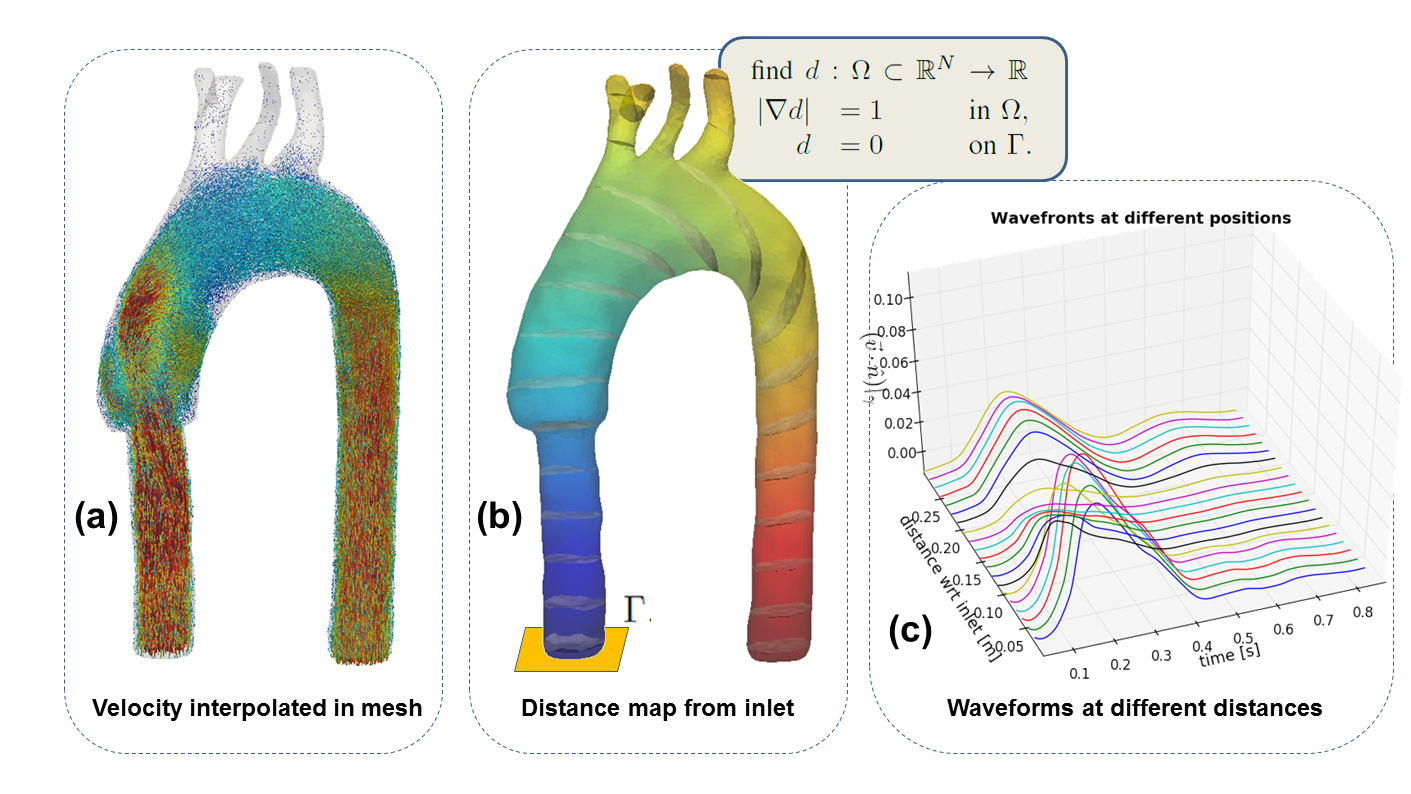
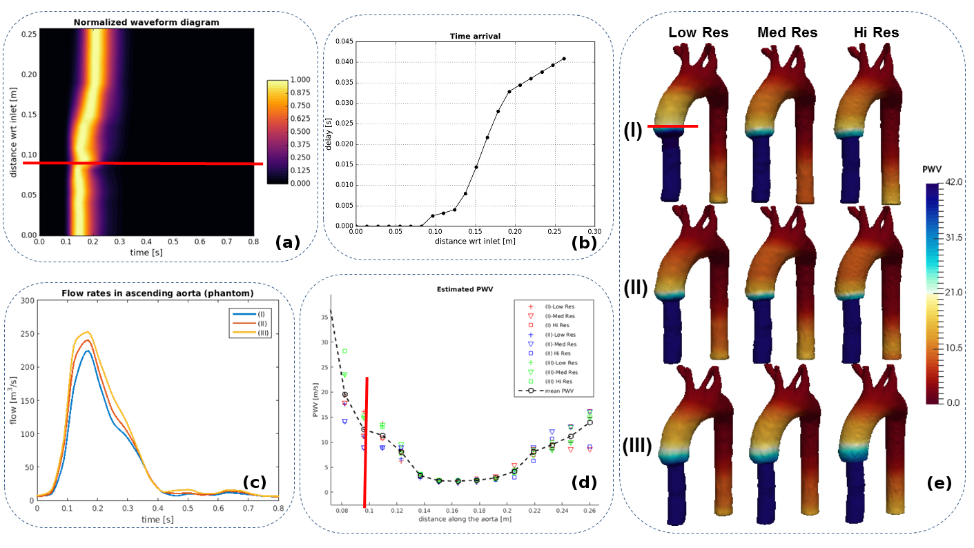
In order to tackle this problem, we solve the distance equation (known as Eikonal equation, see figure 1) in segmented geometries by applying the Fast-Sweeping method for unstructured meshes4. The outcome is a map of the region of interest revealing approximated wavefronts along the artery (since distance do not exactly match -but it is close to- the pulse arrival time), used to calculate local averages of flows with a lower variance to ensure accurate evaluations from 4D-flow data. Once selected a number of isosurfaces from the distance map, we obtain normalized flow waveforms, as in figure 2, used to evaluate the time-delay of PWV along the artery through cross-correlation analysis between one reference curve with respect to the others. Hence, we calculate slowness = 1/PWV = slope of time-delay curve. The latter is obtained by applying linear regressions locally in the curve, due to their sensitivity to noise. Note that slowness is used instead of PWV directly since we may obtain very short delays (almost zero) in some regions. Hence, once obtained the 1D PWV representation, by using the same distance map, we perform the extrapolation of PWV to 3D morphologies in order to facilitate clinical evaluation.Results
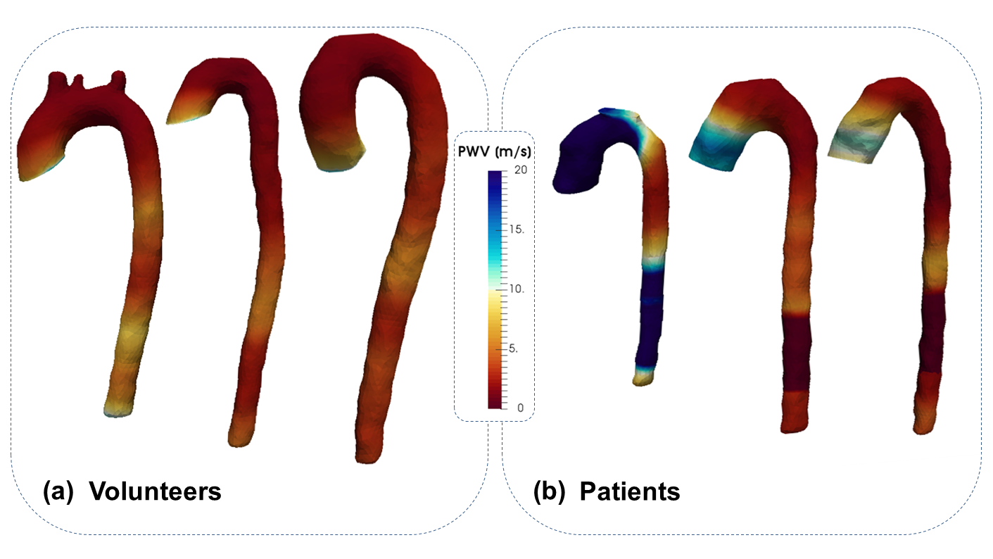
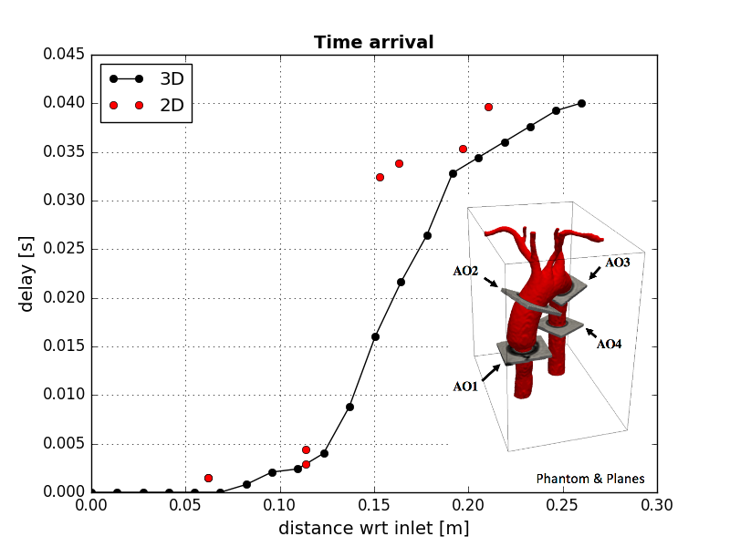
In figure 2, the PWV map estimated in realistic phantom5 from 4D-flow data, using an MR Phillips Achieva 1.5T. The 4D-flow data was collected in three different days (namely I,II,III), and in each one we acquired three different resolutions (namely Low-Res, Med-Res and Hi-Res), showing excellent agreement each other, with a maximum difference below 5% near the section marked with the red line (Figure 2e). We have selected 20 isosurfaces in our evaluations. It can be noticed that appears the stiff tube in blue color, while in the aortic arch it is softer. We must remark that in the case of this phantom, the exact PWV in the tube near the inlet cannot be accurately estimated since there the waves propagates too fast to capture significant variations in cross-correlations with respect to the inlet waveform. Therefore, we have imposed 1/40 [s/m] as the lower limit to slowness to avoid divisions by zero in the calculation of PWV. We also test our method in a set of three volunteers and three Fontan patients, corresponding to figures 3 (a) and (b), respectively. While similar results are obtained in healthy volunteers, where values are between 1 and 8 [m/s], relevant differences can be observed near the aortic arch, where it is expected a stiffer region due to the effect of Fontan disease. On the same patients, several artifacts were observed downstream, mostly due to the movement during the acquisition, since Fontan patients are below 12 years, producing some alterations in our results. In figure 4, we show a preliminary comparison between 2D-flow data collected in four slices, where our method shows a good agreement with the data.Discussion and Conclusion
We present a fast and non-invasive method to estimate PWV in complex geometries. Although preliminary results are quite promising, further validations are still needed. Special attention has to be paid in the determination of the first time arrival since the delay calculated using cross-correlations must increase along the artery, which may fail in evaluations close to the reference isosurfaces or due to noisy data. The application of linear regressions to estimate slopes in time-distance diagrams has been fundamental to deal with realistic inputs. In future developments, we will apply forth and back cross-correlations, as well as an iterative method to recover full 3D PWV considering also local cross-correlations to improve this method.Acknowledgements
We thanks to CONICYT - PIA - Anillo ACT1416, CONICYT FONDEF/I Concurso IDeA en dos etapas ID15|10284, and FONDECYT #1141036 grants. Sotelo J. thanks to the School of Engineering, Pontificia Universidad Catolica de Chile, for his Post-Doctoral Fellow.References
1. Boese JM, Bock M, Schoenberg SO, Schad LR, “Estimation of aortic compliance using magnetic resonance pulse wave velocity measurement”. Phys Med Biol. 2000 Jun; 45(6):1703-13.
2. Grotenhuis HB, Ottenkamp J, Fontein D, Vliegen HW, Westenberg JJ, Kroft LJ, de Roos A, “Aortic elasticity and left ventricular function after arterial switch operation: MR imaging--initial experience”. Radiology. 2008 Dec; 249(3):801-9.
3. Kröner ES, van der Geest RJ, Scholte AJ, Kroft LJ, van den Boogaard PJ, Hendriksen D, Lamb HJ, Siebelink HM, Mulder BJ, Groenink M, Radonic T, Hilhorst-Hofstee Y, Bax JJ, van der Wall EE, de Roos A, Reiber JH, Westenberg JJ, “Evaluation of sampling density on the accuracy of aortic pulse wave velocity from velocity-encoded MRI in patients with Marfan syndrome”. J Magn Reson Imaging. 2012 Dec; 36(6):1470-6.
4. Qian J, Zhang YT, Zhao HK, “Fast sweeping methods for Eikonal equations on triangular meshes”. SIAM J. Numer. Anal. 2007; 45(1):83-107.
5. Urbina J, Sotelo JA, Springmüller D, et al. Realistic aortic phantom to study hemodynamics using MRI and cardiac catheterization in normal and aortic coarctation conditions. J Magn Reson Imaging. 2016 Sep;44(3):683-97
Figures