Synopsis

Real-time B0 feedback has been shown to be beneficial for the controlling of B0 fluctuations. However, update rates that have been reported are slow (~100ms) and either use pre-emphasis to correct for the coupling and faster dynamics of the system or only use control the frequency

We show that for faster update rates (±1ms) pre-emphasis (i.e. dynamic decoupling) is not required and that static decoupling can perform equally well or better.

Introduction

The static B0 magnetic field of MRI scanners can be measured with high-temporal resolution using NMR field cameras. Using this method, real-time feedback has been shown to be beneficial for the controlling of B0 fluctuations^1-3. However, update rates that have been reported are slow (~100ms) and either use pre-emphasis to correct for the coupling and faster dynamics of the system^1,2 or only use control the frequency³.

In this work, we show that for faster update rates (±1ms) pre-emphasis (i.e. dynamic decoupling) is not required and that static decoupling can perform equally well or better. This design method applies to both spherical harmonic shimming and multi-coil B0 setups⁴.

Theory

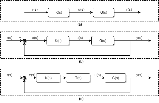
Typical feedback control systems are shown in Fig. 1. For linear time-invariant systems, the system that needs to be controlled can be represented as a transfer function G(s). The system usually needs to be identified (characterised) so that the behaviour of the system can be approximated. This is done by measuring the output y(s) by applying a known input u(s) and modelling G(s)^5-7.

The controller K(s) needs to be designed such that the closed-loop response y(s) is stable, robust and has good performance. An industry standard is to use propertional-integral (PI) controllers that have the form^1,8:

$$K(s) = K_P + K_I/s$$

These controllers are easy to implement and have many different tuning strategies. For multivariable systems, G(s) has multiple inputs/outputs. Decoupling is a method that tries to minimise cross-interactions and convert the system into single-input single-output (SISO).

Methods

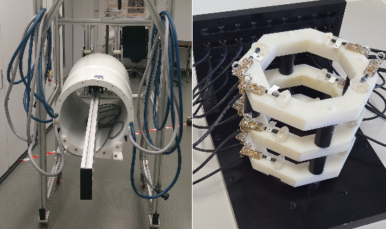
The shim system G(s) was a 28 channel insert shim from Resonance Research Inc. (Billerica, MA) that included 0^th, 2^nd, 3^rd and 4^th degree spherical harmonic terms (Fig. 2). The measurements were performed on a 9.4T Siemens whole-body human MRI scanner (Erlangen, Germany).

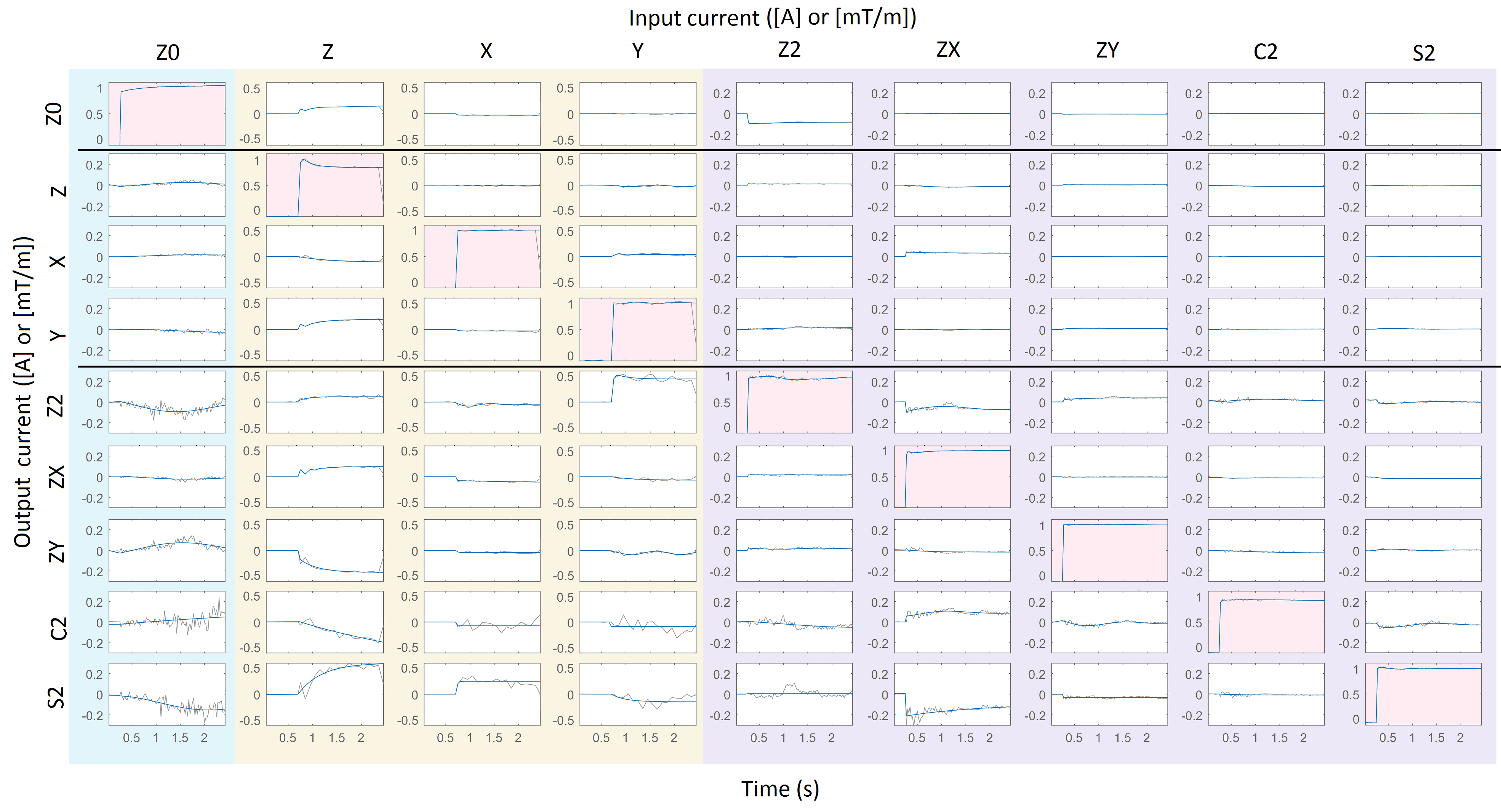
System identification was performed in the time-domain using step inputs of 1.0A as inputs to each shim channel and 1mT/m to each gradient. An instrument variable method was used to estimate the transfer functions⁹. The outputs of the system (magnetic field) were measured using a custom built ¹H NMR field camera¹⁰ with TR = 25ms (Fig. 2). The outputs y(s) were the field coefficients obtained using spherical harmonic decomposition. All shim channels up to 4^th degree were characterized. For proof of concept, only shim terms up to 2^nd degree were used, so up to 2^nd degree field coefficients were used for decomposition. Thus, the system had 9 inputs and 9 outputs.

A static and dynamic decoupling strategy for controller design were compared. The dynamic decoupling was performed using an inversion method with pole/zero mirroring and a propering filter to keep the system stable¹¹. Dynamic decoupling is similar to pre-emphasis^12-14. The static decoupling was done by inverting the steady-state values. The decoupling strategies were analysed using the mu-interaction¹⁵:

$$μ_∆ ((P_d (ω)-diag{P(ω)})(diag{P_d (ω)})^{-1})$$

where is the frequency response function (FRF), is the FRF of the decoupled system and denotes the largest singular value of the decoupling controller Δ. This interaction measure has a direct relationship to the robustness of the decoupled system¹⁵.

Optimised PI controllers were designed for each SISO self-term by minimising the open-loop phase margin (to optimise robustness) and constraining the integral-absolute-error to be less than 0.003. The controllers were converted to discrete-time using the Tustin transform and the sampling rate was assumed to be 1ms.

Results and Discussion

The system measurements and model are shown in Fig. 3. The models had an accuracy of at least 60% for off-diagonal terms and more than 90% for diagonals.

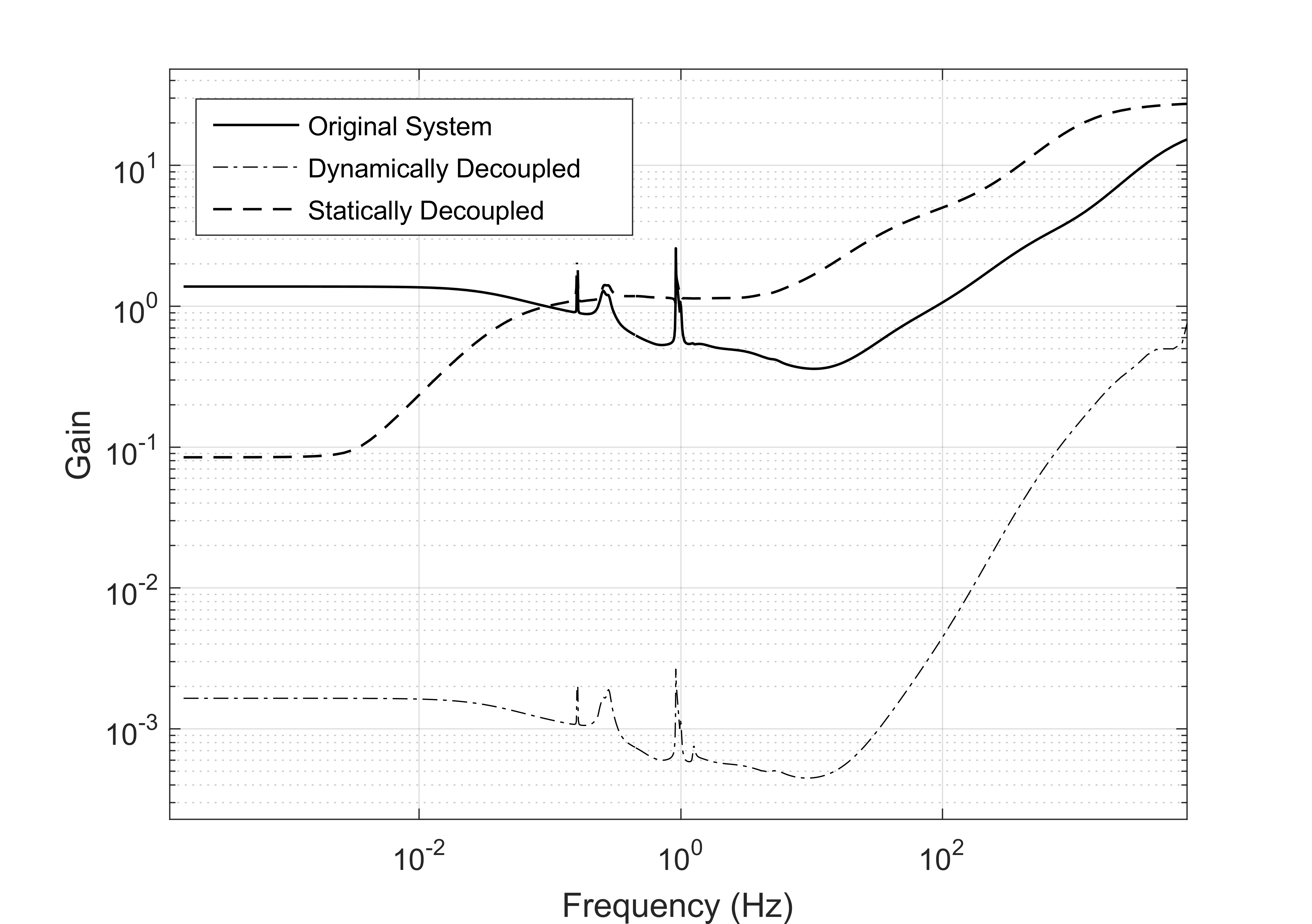
As expected, the dynamic decoupling has much lower mu-interaction as it decouples the system much better than the static decoupling (Fig. 4). However, the static decoupling decouples the system very well at low frequencies and is better than the original system up to approximately 5kHz.

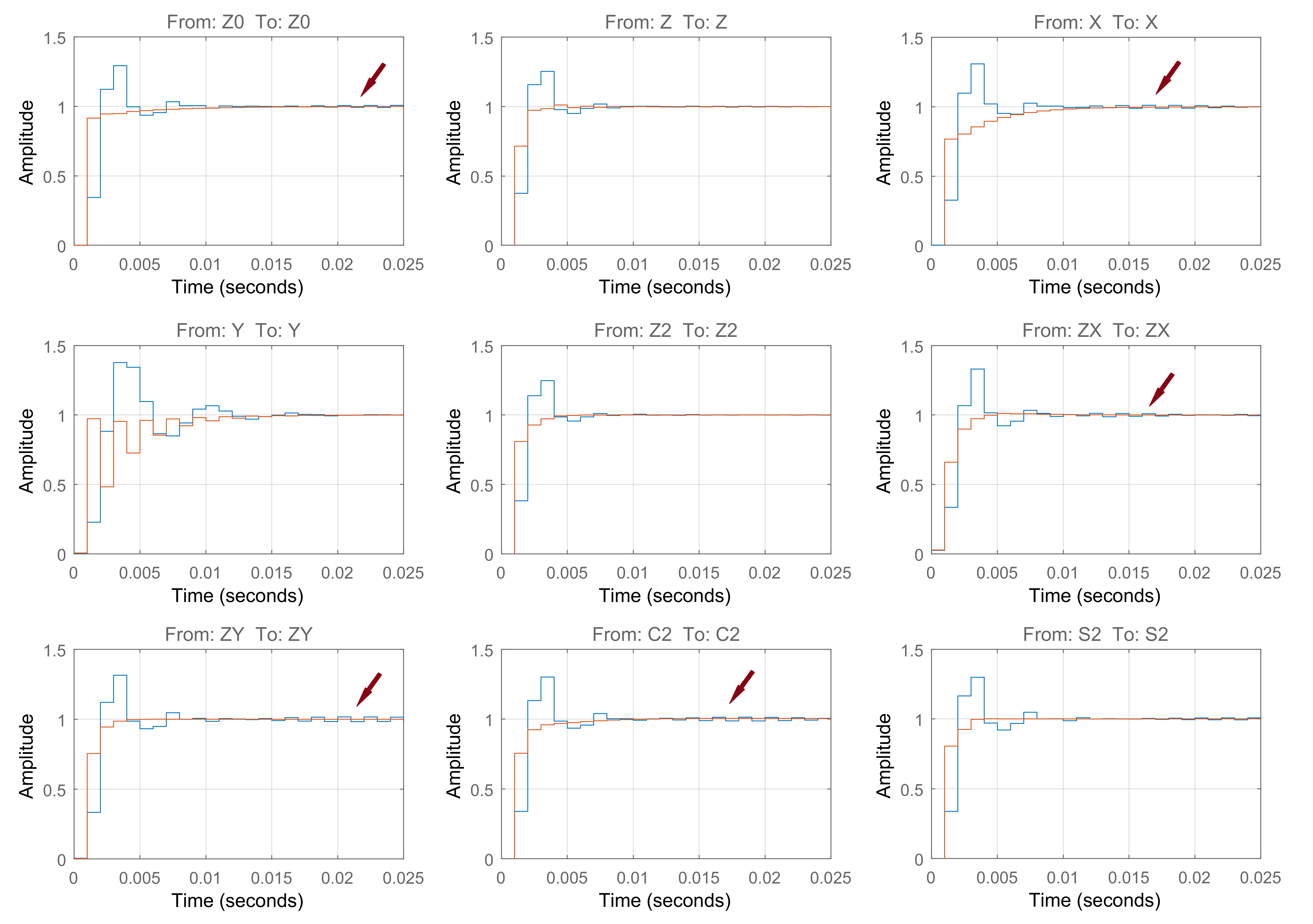
Combined with the PI controllers, the two decoupling methods are very similar in performance (Fig. 5). However, due to the high frequency performance of the dynamic decoupling and the discretisation of the system, “ringing” is introduced in the output (Fig. 5). This results in compromised robustness, which is higher for static decoupling.

Conclusion

We characterised a 2^nd, 3^rd and 4^th degree shim system using a custom-built NMR field camera at 9.4T. Different decoupling control methods were investigated in a proof of principle study using only the 2^nd degree system. Static or dynamic decoupling (i.e. preemphasis) achieve similar performance and robustness using feedback control. However, for discrete-time controllers, dynamic decoupling may yield undesirable “ringing” in the system.

Acknowledgements

References

[1] Duerst Y et. al. MRM 2015.

[2] Wilm B et al. MRM 2014.

[3] Boer V et al. MRM 2012.

[4] Juchem C et al. JMR 2011.

[5] Oppenheim AV and Schafer RW. Digital Signal Processing (3rd ed). 2014.

[6] Vannesjo SJ et. al. MRM. 2013.

[7] Vionnet L et. al. Proc. of ISMRM 2016.

[8] Astrom KJ et. al. Instr., Sys. and Automation Soc. 1995.

[9] Young PC and Jakeman AJ. Intl. Jour. of Control. 1980.

[10] Barmet C et al. MRM. 2008.

[11] Hess RA and Siwakosit W. Jour. of Aircraft. 2001.

[12] Edler K and Hoult D. MRM. 2008.

[13] Juchem C et. al. Concepts in MR (B). 2010.

[14] Fillmer A et. al. MRM. 2015.

[15] Grosdidier P and Morari M. Automation. 1986.