2651
Validation of RF-induced temperature increase in a phantom: comparison of numerical simulations, MR thermometry and measurements from temperature sensors.1Laboratory for Cognitive Brain Mapping, RIKEN Brain Science Institute, Saitama, Japan, 2Research Resources Center, RIKEN Brain Science Institute, Saitama, Japan
Synopsis
In this study, we compared the temperature increase calculated by the simulations and measured by the MR-thermometry in a phantom with those measured by the optical temperature sensors, with good agreement between the methods. To ensure safety, IEC guidelines require simulations of SAR along with validation in phantoms. While it is likely impossible to simulate every possible pulse shape and phase combination in a pTx system with a large number of transmit channels, the results we present here suggest that simulations plus MR-thermometry could provide the verification currently lacking in pTx studies.
Purpose
During MR imaging the radiofrequency pulses cause heating and during a parallel transmission (pTx) MRI, it becomes hard to predict the local hot spots. To ensure subject safety, the IEC guidelines1 recommend, precise modeling of pTx array and calculation of EM fields and SAR values should be done and must be validated at least in a phantom. This study is performed to validate the temperature increase calculated by the numerical simulations and measured by the MR thermometry2 (ΔT-Imaging) in an agar gel phantom by comparing them with those measured by the optical temperature sensors (T-sensors). While it is likely impossible to simulate every possible pulse shape and phase combination in a pTx system with a large number of transmit channels, the results we present here suggest that simulations plus ΔT-Imaging could provide the verification currently lacking in pTx studies.Methods
A 2-channel transmit-receive array with a radius of curvature of 85mm (Figure-1a) was built, to be used with an Agilent 4T-MRI scanner. An agar gel phantom (15g/L agar, 4.0g/L NaCl, 0.02g/L MnCl2) was prepared in a cylinder (OR = 65mm, IR = 59mm, L = 200mm). Another cylinder (OR = 15mm, IR = 9mm, L = 200mm) was placed eccentrically inside the phantom and was filled with lard (figure-1b). Four T-sensors (Luxtron-790) were placed inside the gel at different locations to measure the temperature increase (Figure-1c).
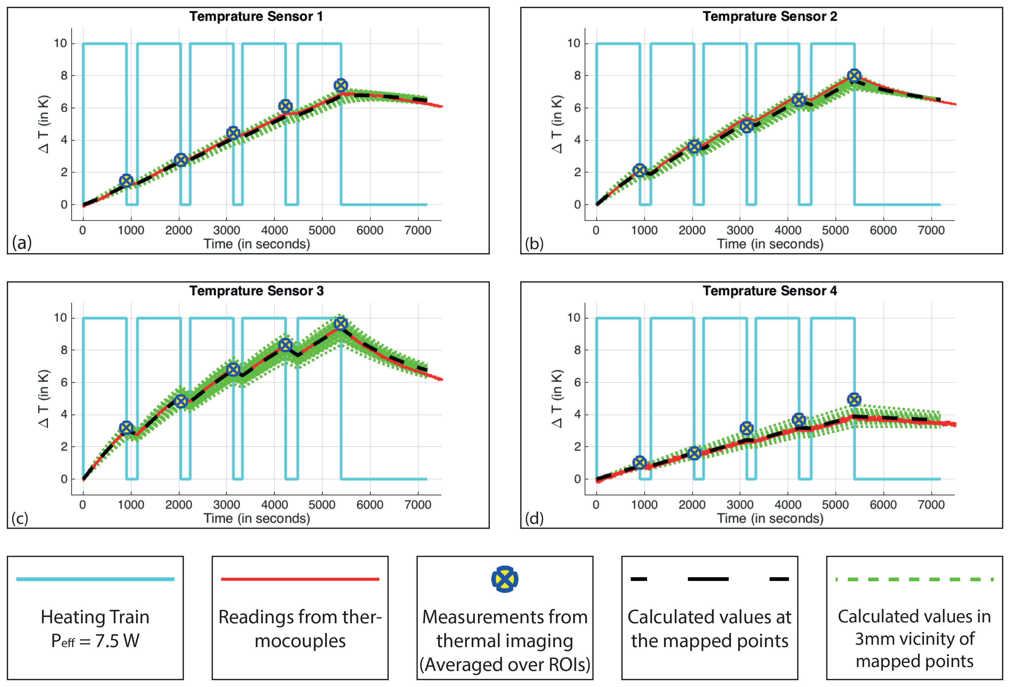
The phantom was heated using only one of the coils (ch-1) with a square wave pulse (1.5ms pulse; 10ms TR; Power = 50W; Effective Power ($$$P_{eff}$$$) = 7.5 W) for 15 minutes before performing MR thermometry. Five such cycles were performed (Figure-2). Power dissipated in to the phantom by ch-1 was calculated using S-parameters, to be 82% of $$$P_{eff}$$$.
For ΔT-Imaging (PRF shift method2), an asymmetric spin echo pulse sequence was used ($$$TE$$$ = 35.7ms, $$$TE_{eff}$$$ = 12ms; resolution = 3mm isotropic). Temperature change maps were calculated using
$$\Delta T = \frac{\varphi_{w} - \varphi_{f}}{2\pi f_{0}\alpha TE_{eff}}$$
where $$$\Delta T$$$ is the temperature change, $$$\varphi_{w}$$$ and $$$\varphi_{f}$$$ are the phase shifts from agar gel and lard respectively, $$$f_{0}$$$ is 170.33MHz, $$$\alpha$$$ is the thermal proton resonance frequency change coefficient. For the agar gel, $$$\alpha$$$ of -0.0135ppm/K was used, which was determined from an independent experiment. The temperature increases were averaged over regions of interest (ROIs) near the tip of the T-sensors.
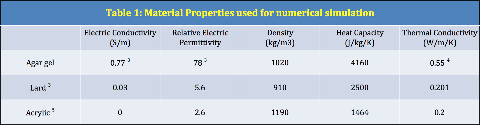
Numerical simulations were performed using CST Studio Suite® 2016 (CST AG, Darmstadt, Germany). The Time Domain Solver in CST Microwave Studio® was used for electro-magnetic simulations and Thermal Transient Solver in CST Mphysics Studio® for thermal simulations. Material properties used for the simulations are given in Table-1. T-sensor tips were manually mapped to the simulations. For each mapped T-sensor point, temperature increases were also calculated on the vertices and the face centers of the cubes (1mm3, 8mm3, 27mm3) enclosing that mapped point at their center.
Results
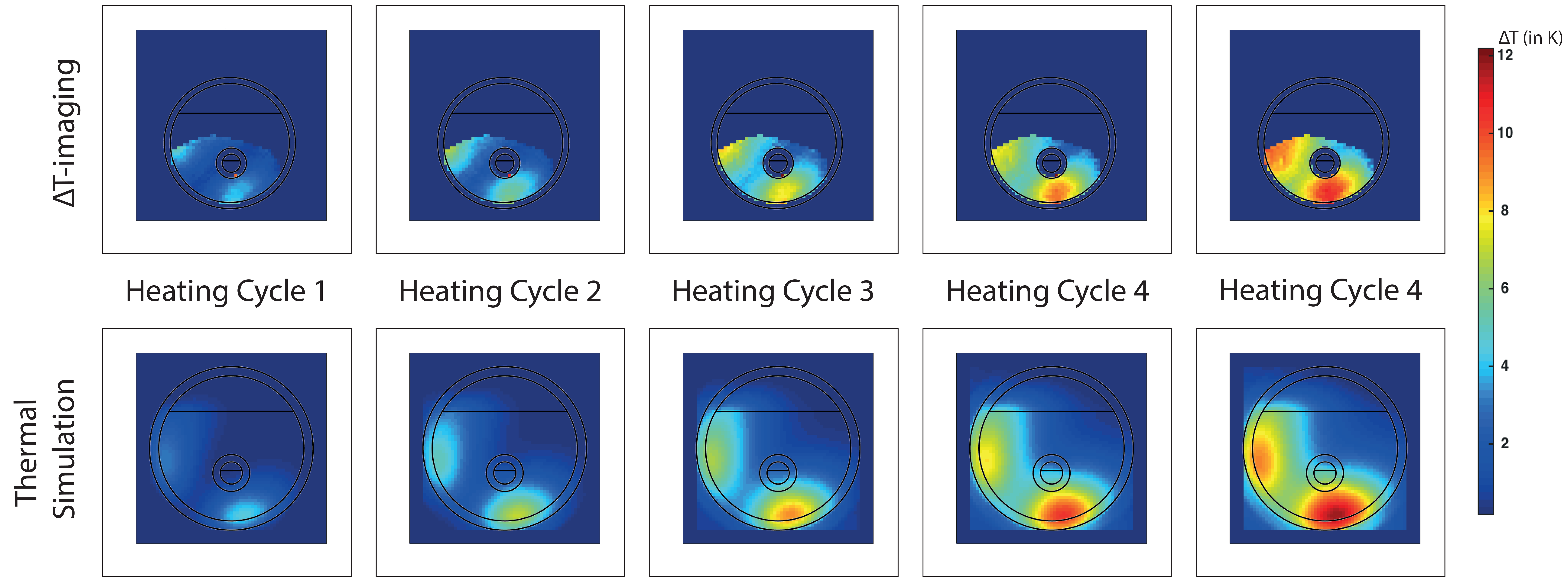
Figure-2 shows that the increase in temperature recorded from each of the four T-sensors, the measured values from the ΔT-Imaging and the values calculated from the numerical simulations are in good agreement. The standard deviation (StDev) of the differences between the T-sensor readings and ΔT-Imaging are 0.23, 0.19, 0.23 and 0.41 and the StDev of the differences between the T-sensor readings and calculated values are 0.1, 0.13, 0.11 and 0.08. StDev of T-sensor-4 and ΔT-imaging is higher than others because the T-sensor-4 happened to be placed in a region where SNR was very low. Figure-3 shows the similar patterns of temperature increase for the center slice from ΔT-imaging and simulation at the end of each heating cycle.Discussion and Conclusion
This study has shown that for in-homogeneous heating in a phantom, the T-sensor readings, the measured values from the ∆T-Imaging and the simulated temperature changes are in good agreement. As mentioned above, IEC guidelines1 require simulations of SAR along with validation in phantoms. In practice, pTx RF pulse parameters are determined after the subject is placed in the magnet, making phantom validation of the actual pulse parameters nearly impossible. While ∆T-Imaging lacks the precision2, to confirm compliance with IEC SAR limits, our results suggest that it could serve as a real-time confirmation of the simulations, identifying any inconsistencies with the simulations before actual tissue damage occurs (at 43°C).Acknowledgements
This work was partially funded by the “Brain Mapping by Integrated Neurotechnologies for Disease Studies” (Brain/MINDS) by the Ministry of Education, Culture, Sports, Science and Technology of Japan (MEXT).References
1. IEC 60601-2-33. March 2010:1-224. http://ieeexplore.ieee.org.
2. Streicher MN, Schäfer A, Ivanov D, et al. Fast accurate MR thermometry using phase referenced asymmetric spin-echo EPI at high field. Magn Reson Med. 2014;71(2):524-533.
3. Zhang M, Che Z, Chen J, et al. Experimental Determination of Thermal Conductivity of Water−Agar Gel at Different Concentrations and Temperatures. J Chem Eng Data. 2011;56(4):859-864.
4. Hasgall PA, Di Gennaro F, Baumgartner C, et al. IT’IS Database for thermal and electromagnetic parameters of biological tissues. Version 2.6, January 13th. 2015. 2015;3(1):11-15. doi:10.13099/ViP-Database-V2.6. Accessed January 23, 2016
5. Physical Properties Table for Acrylic. 2016. https://www.hazaiya.co.jp/category/bussei_pipe.html. Accessed February 12, 2016
Figures
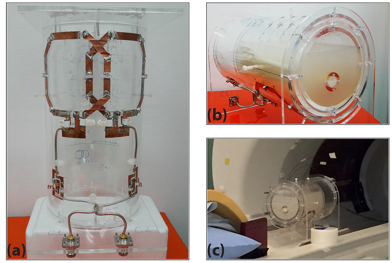
Figure-1: (a) The two-channel transmit-receive surface coil array. Surface coils were tuned and matched to 170.33MHz and were overlapped for decoupling (S11 = -23dB, S21 = -16dB, S12 = -16dB & S22 = -27dB). (b) Arrangement of the coil, the agar gel and the lard. The lard tube placed in sagittal plane close to the coil. (c) Arrangement of thermometers. At the top of the coil housing and phantom, holes were made at marked places to insert thermometers.