2555
Conversion of Brain Tissue volumes by MR Images form 1.5 to 3.0 Tesla scanners for Multiple Sclerosis patients1University of Sao Paulo, Ribeirao Preto, Brazil
Synopsis
Brain tissue volume estimation based on MRI is crucial to several diseases such as multiple sclerosis (MS). The Images from different scanners with dissimilar magnetic fields have disparities in resolution, Signal to Noise Ratio, contrast, among others. In order to convert volume estimations from different scanners, we suggest and evaluated two methods. The dataset to validate the methods was selected from 14 years follow up study of 72 MS patients with 1.5 and 3.0 Tesla acquisitions. The quantitative study of tissue volume progress is possible using these two methods.
Materials and Methods
Multiple sclerosis (MS) is the most common immune-mediated demyelinating disease of the central nervous system1. While much work has concentrated on focal White Matter (WM) lesions in MS, there is growing evidence to suggest that Grey Matter (GM) are also involved in the disease process2. So analyzing the volume of tissues is a way to interpret the progress of MS.
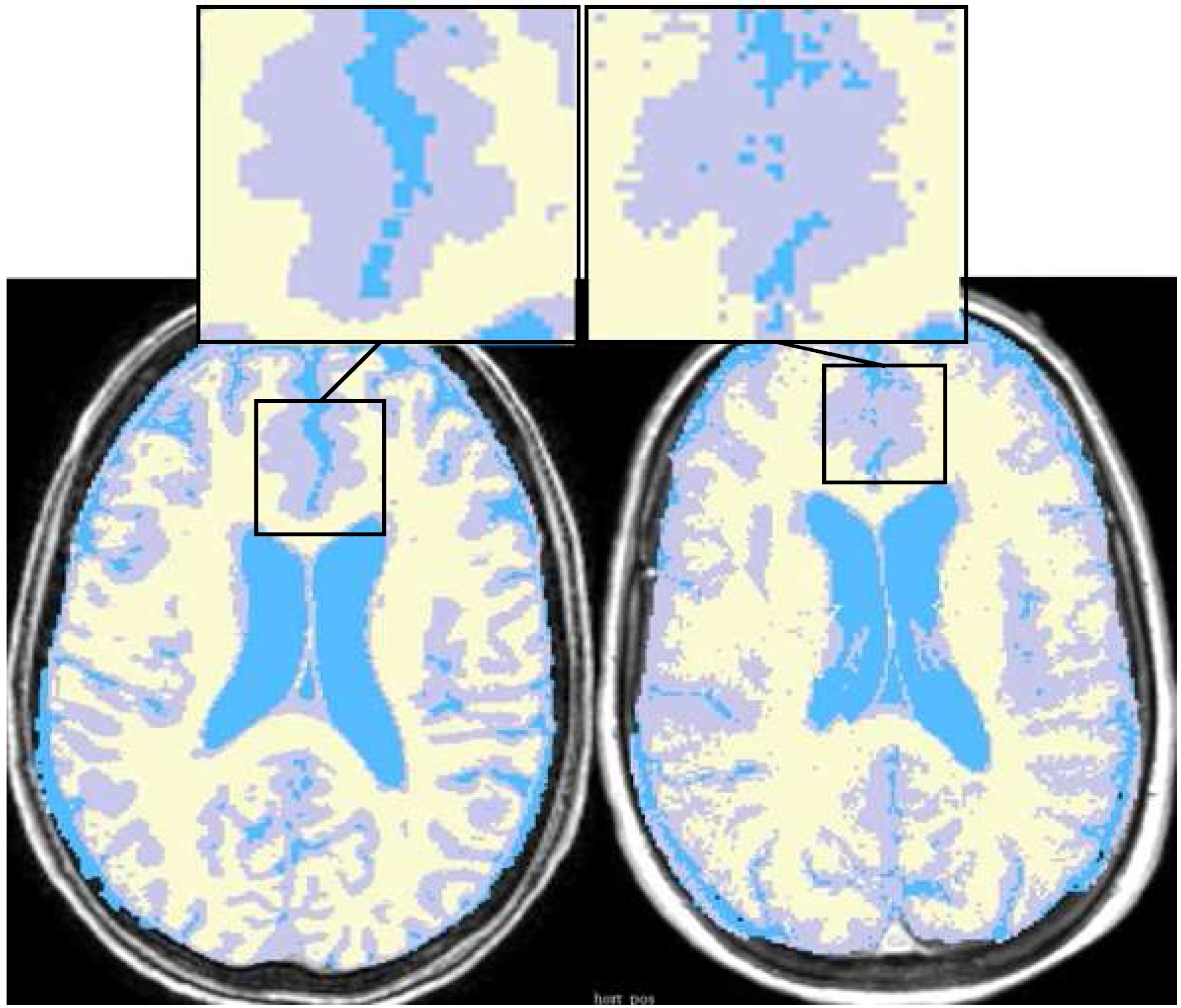
In order to convert the estimation of volume of a tissue from 1.5 to 3.0 Tesla, ten persons are chosen to be scanned in both 1.5 and 3.0 Tesla in the same day similar to previous study3. The segmentation algorithm for measuring the volumes provided by the 3DSlicer module4 is hierarchical EM algorithm5 which showed good results respect to other software. Example of simple segmentations both on 1.5 and 3.0 Tesla can be seen in Figure 1.
Data Analysis
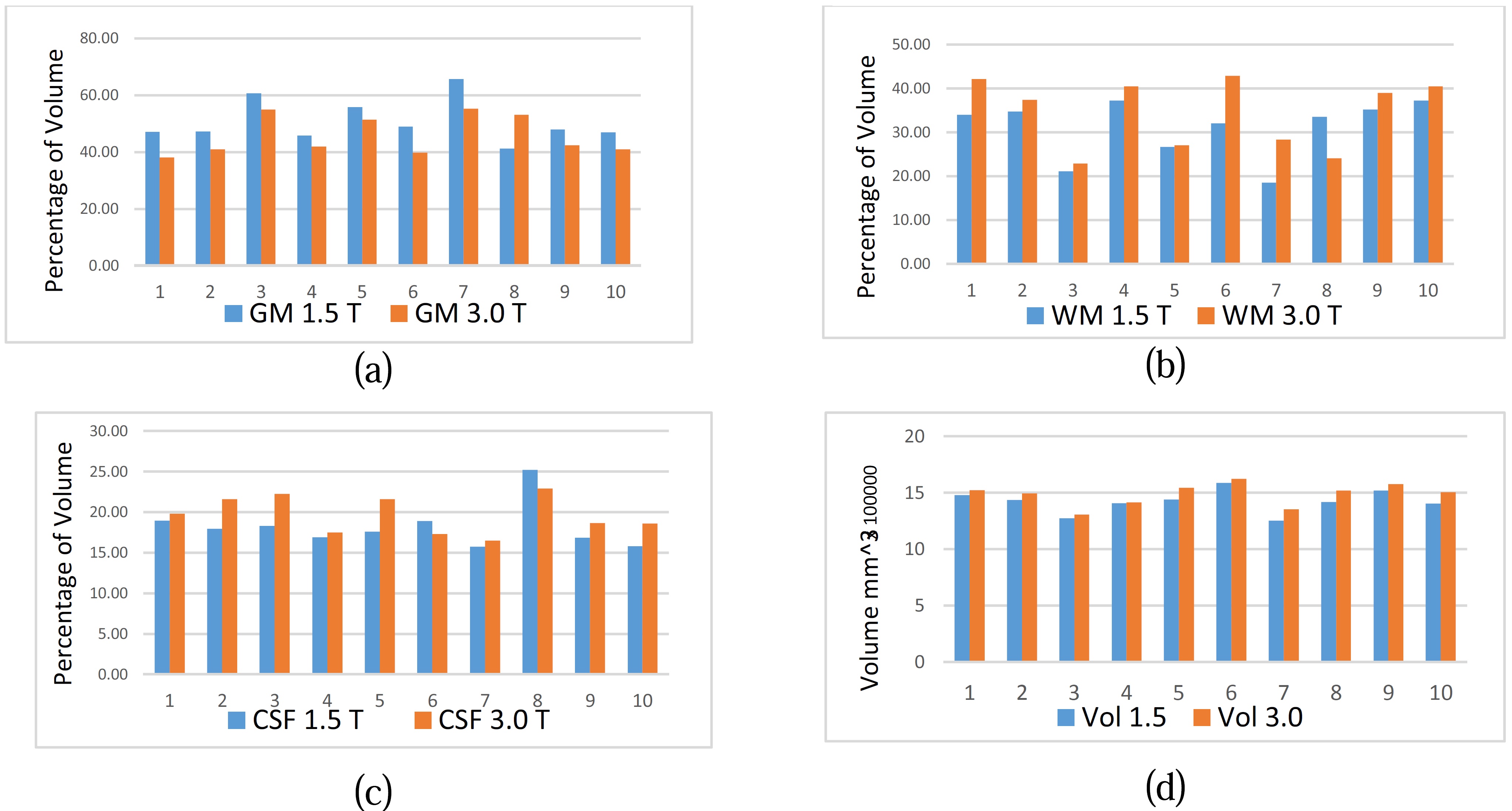
By segmenting and measuring the volume of tissues of those ten samples, Histogram 1 shows changes in GM, WM, CSF and total volume between two kinds of MRIs (1.5 and 3.0 Tesla). Although it is needed to consider all factors, which have effects on changes3 in this work we just focused on graphical and mathematical parts. If we precisely look at some part of images, it seems that a part of GM is inside WM and a part of CSF is inside the GM and vice of versa (see overlapping in Figure 1). Therefore we suggest a general graphical model which is a linear equations system $$ \widetilde{GM_{3.0}}=GM_{1.5}+\alpha_{1}.WM_{1.5}+\beta_{1} .CSF_{1.5}+\gamma_{1}.Vol$$ $$ \widetilde{WM_{3.0}}=WM_{1.5}+\alpha_{2}.GM_{1.5}+\beta_{2} .CSF_{1.5}+\gamma_{2}.Vol (1)$$ $$ \widetilde{CSF_{3.0}}=CSF_{1.5}+\alpha_{3}.WM_{1.5}+\beta_{3} .GM_{1.5}+\gamma_{3}.Vol$$ where $$$ \widetilde{A}$$$ is converted tissue $$$A$$$, $$$GM_{1.5}$$$is the volume of $$$GM$$$ in 1.5 Tesla image and so on and$$$Vol$$$ is amount of total volume in 1.5 Tesla image. Next step is to obtain coefficients$$$\alpha_{i}, \beta_{i}$$$ and $$$\gamma_{i}, i=1,2,3$$$. As we can see system (1) has three equation with nine unknowns variables. Fortunately there are some graphical information about coefficients which help us to find a solution for system (1). By using the average of increasing in volume for those nine patients we have $$\gamma_{1}+\gamma_{2}+\gamma_{3}= C_1 \ (2)$$ where $$$C_1$$$ is known. Also we have $$\alpha_{1}.WM_{1.5}=\alpha_{2}.GM_{1.5}$$ $$\beta_{1}.CSF_{1.5}=\beta_{3} .GM_{1.5} (3)$$ Because of the high difference between the gray level of CSF and WM we can ignore the overlapping between CSF and WM. It means $$\alpha_{3}\cong 0 \ (4)$$ consequently $$\beta_{2}\cong 0 \ (5)$$ In addition, we can let $$\gamma_{2}=\gamma_{3}\cong 0 \ (6)$$ because growing volume is just for exterior layer which is GM. Now by using equations (2)-(6), system (1) will be reduced to $$ \widetilde{GM_{3.0}}=GM_{1.5}-\alpha.GM_{1.5}-\beta.GM_{1.5}+\gamma.Vol$$ $$ \widetilde{WM_{3.0}}=WM_{1.5}+\alpha.GM_{1.5} \ (7)$$ $$ \widetilde{CSF_{3.0}}=CSF_{1.5}+\beta.GM_{1.5}$$ where the sign of coefficients obtained from Histogram 1. Since $$$\gamma= C_1$$$ clearly first equation in (7) depends on two others so we have just two equations and two unknowns $$$\alpha $$$ and $$$\beta $$$. Then $$\alpha =\frac{\widetilde{WM_{3.0}}- WM_{1.5}}{ GM_{1.5}}=C_2$$ $$\beta =\frac{\widetilde{CSF_{3.0}}- CSF_{1.5}}{ GM_{1.5}}=C_3$$ These $$$\alpha $$$ and $$$\beta $$$ can be calculated for all nine patients averagely (by substituting $$$WM_{1.5}$$$ for $$$\widetilde{WM_{3.0}}$$$ and so on). Therefore system (7) with calculating coefficients by using above information, is one suggestion to convert volumes. In addition to this model based method, linear interpolation is proposed as another method.Numerical results
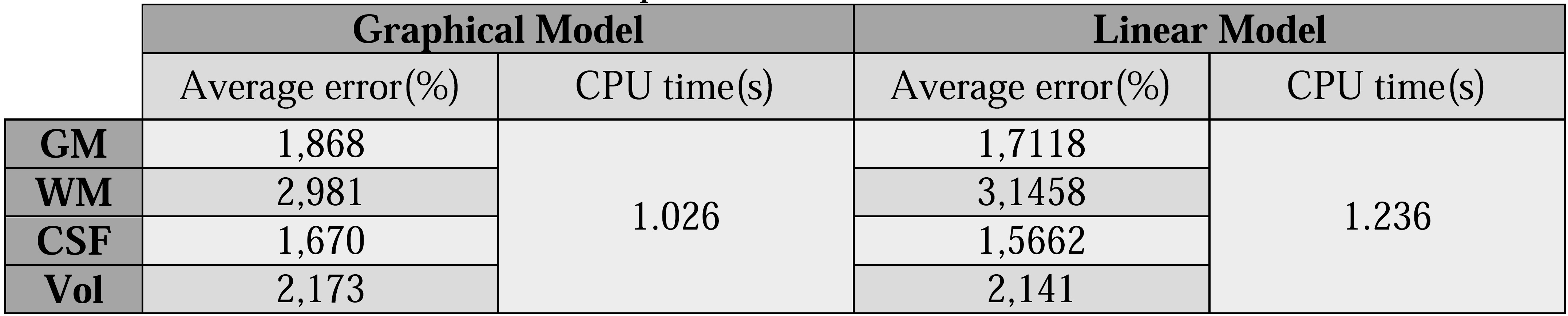
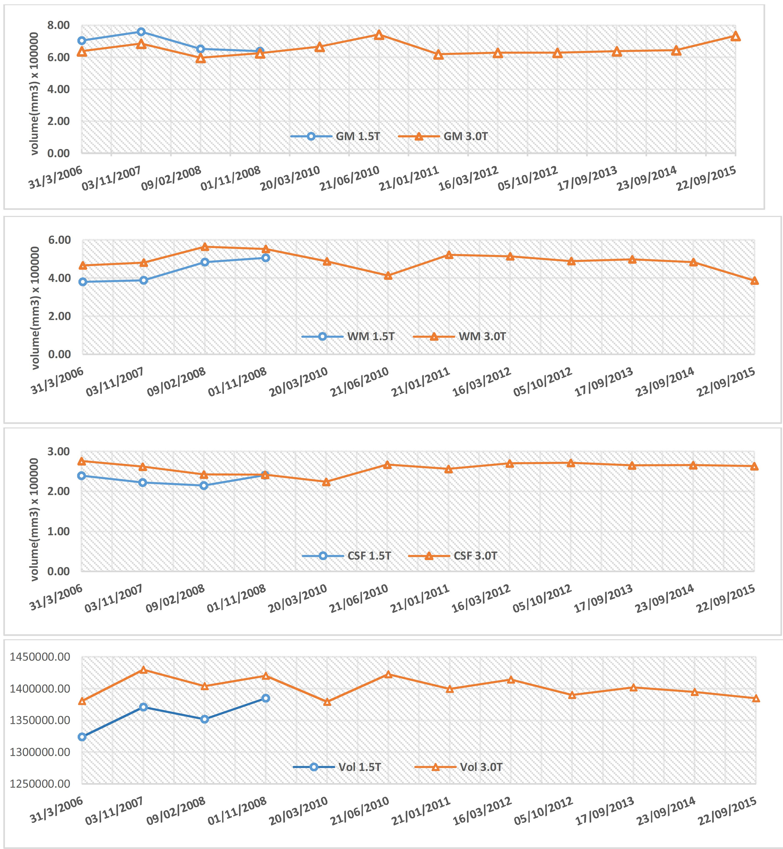
After introducing two methods to convert the volume of tissues for 72 patients with MS disease we segmented all of their images during the treatment which was around 14 years and totally the number of segmented MRIs were 472 images. Relative error is used for showing the accuracy of models $$\epsilon=\frac{\mid\widetilde{T}-T\mid}{Vol}$$ which $$$\widetilde{T}$$$ is converted volume of tissue, $$$T$$$ is measured volume of tissue in 3.0 Tesla and $$$Vol$$$ is total brain volume in 3.0 Tesla MRIs. Relative errors have been calculated and presented in Table 1 for different methods. In Graph 1 we can see the whole variation of tissue volumes in one figure simultaneously converted and original measurements for one of patients.Conclusion
In this study, for the problem which was how different data from two kinds of MRI scanners can be used and interpreted in one plot, two methods were suggested. The methods for converting the volumes from 1.5 to 3.0 Tesla were tested and the results and errors presented. The selected method to convert volumes from all (72) patients can be Graphical model or Linear model. Depends on interested tissue in brain one method may show better result than the other. All the results are tested by 3DSlicer software and EMSegmenter method. The comparison between software for segmentation, modifying the algorithm and evaluation of our method using phantoms are our future works.Acknowledgements
This research was supported by CAPES agency. We thank our colleagues from FFCLRP and CCIFM who provided insight and expertise that greatly assisted the research, although these collaboration still continues.References
1. Gaindh D., Kavak K. S., Teter B., Vaughn C. B., Cookfair D., Hahn T., Weinstock-Guttman B. and N. Y. S. M. S. Consortium, Journal of the Neurological Sciences 370, 13-17 (2016).
2. Chard D., Griffin C., McLean M., Kapeller P., Kapoor R., Thompson A. and Miller D., Brain 125 (10), 2342-2352 (2002).
3. Lysandropoulos A. P. , Absil J., Metens T., Mavroudakis N., Guisset F., Van Vlierberghe E., Smeets D., David P., Maertens A. and Van Hecke W., Brain and behavior (2016).
4. Teams D., https://www.slicer.org/slicerWiki/index.php/Documentation/3.6 (2013).
5. Pohl K. M., Bouix S., Nakamura M., Rohlfing T., McCarley R. W., Kikinis R., Grimson W. E., Shenton M. E. and Wells W. M., IEEE transactions on medical imaging 26 (9), 1201-1212 (2007).
Figures