2423
A simple partial volume correction method for magnetization transfer ratio images1Lysholm Department of Neuroradiolgy, National Hospital for Neurology and Neurosurgery, London, United Kingdom, 2Academic Neuroradiological Unit. Dept. of Brain Repair and Rehabilitation, University College London, United Kingdom, 3Sydney Neuroimaging Analysis Centre, Sydney, Australia, 4Academic Neuroradiological Unit. Dept of Brain Repair and Rehabilitation, University College London, United Kingdom, 5National Prion Clinic, National Hospital for Neurology and Neurosurgery, United Kingdom, 6MRC Prion Unit. Department of Neurodegenerative Diseases, UCL Institute of Neurology, United Kingdom
Synopsis
We here demonstrate how partial volume correction by linear regression in the style originally proposed for arterial spin labelling MRI can be used to perform a simple and effective partial volume correction for Magnetisation Transfer Ratio data.
Introduction and Purpose
Magnetisation transfer (MT) acquisitions provide extremey valuable information, most notably for Multiple Sclerosis [vanBuchem1997].The extraction of tissue specific parameters can be confounded by the limited spatial resolution of the images; the partial volume (PV) errors arising from averaging between neighbouring tissues has been discussed early on for MT [Kalkers2001]. With 2D readouts with typical slice thickness of 2-3mm, not sufficient to easily discriminate the contribution to the signal of different tissue types. Methods have recently been suggested to remove the cerebro spinal fluid contamination of the estimated parameters when using quantitative MT protocols by extending the conventional 2-pool model [Deoni2013, Mossahebi2014]. However, for single-offset MT weighted or MT ratio (MTR) acquisitions, when using histograms , the most commonly employed method to reduce PV effects is thresholding partial-volume probability maps [Dehmeshki2003]. However the results are likely to be affected by the threshold chosen, and thecortical ribbon may end up excessively thin. We demonstrate how partial volume correction by linear regression in the style originally proposed for arterial spin labelling MRI [Asllani2008], can be used to perform a simple effective partial volume correction for MTR data.
Methods
As proof of principle for this methodology we selected data from 2 subjects enrolled in the UK National Prion Monitoring Cohort, who expressed their informed consent for the study: a 34-year old healthy subject and a 50-year year old patient with inherited prion disease.
MRI. Siemens 3T Tim Trio, 32-channel head coil. Structural imaging (T1w): 3D-MPRAGE, TR=2200ms, TE= 2.9ms, TI=900ms, flip angle (α) 10°, 208 partitions, (1.1mm)^3 resolution). MT measurement: 3D-FLASH with/without presaturation pulse (10ms Gaussian, 1200Hz offset, α=500°), yielding Msat (partially saturated) and M0 (equilibrium) images; TR=42ms, TE=3ms, α=5°, (22.2cm)^2 FoV and an unisotropic spatial resolution of 0.9mm in plane and 3mm in the ‘slice’ direction (60 partitions).
Data Processing. T1w data was simultaneously segmented and regional labels estimated using a joint multi-atlas and Gaussian mixture model method [Cardoso 2015], then affine-registered to the Msat dataset using nifty_reg [Ourselin 2001]. Fractional probability maps for grey, white matter and CSF (pGM, pWM, pCSF) were also downsampled to the MT data space using a point spread function method [Cardoso 2015b]. The M0 data was rigidly registered to the Msat data before computing MTR maps as 1-Msat/M0.
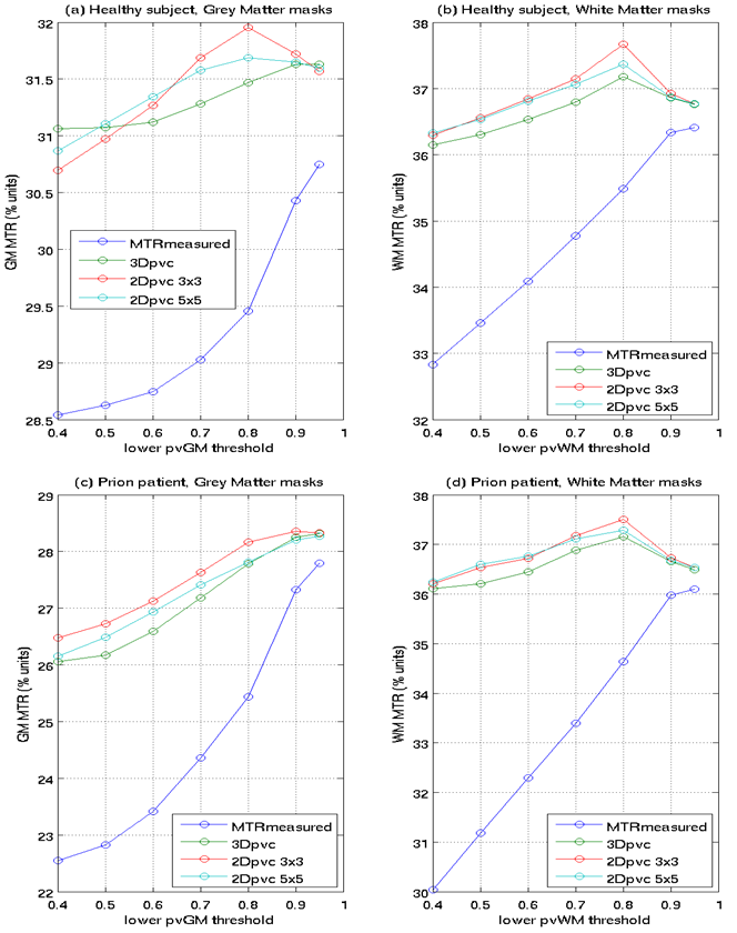
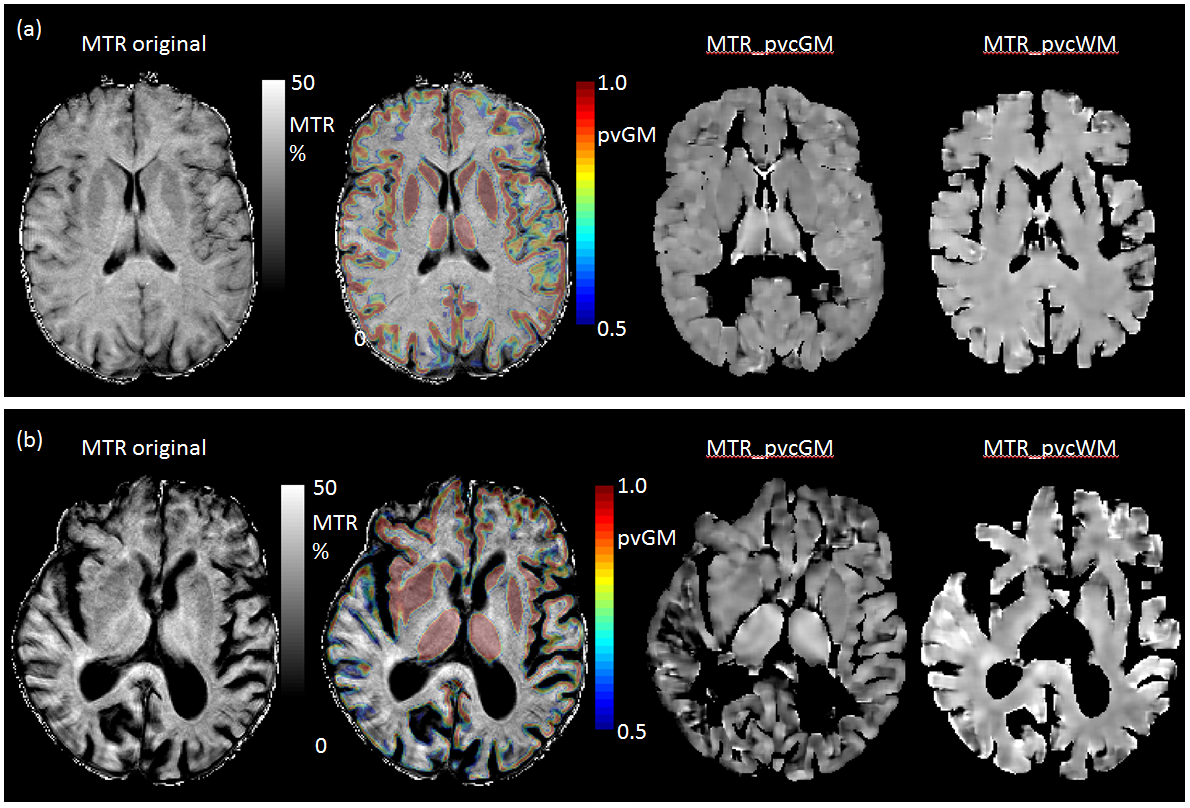
PV correction. For PV correction we used the linear regression algorithm described in [Asllani 2008]: the equation MTR_measured=pGM*MTR_GM + pWM*MTR_WM + pCSF*MTR_CSF) is solved over a 2 dimensional kernels of 3x3 or 5x5 voxels or a 3D kernel (3x3x3) assuming local tissue-specific MTR values do not change within the voxel; it is thus possible to obtain PV corrected (pvc) estimates of MTR_GM and MTR_WM (MTR_ pvcGM, MTR_ pvcWM-) voxel-by-voxel. To illustrate the benefits of the PV correction, masks are generated for pvGM and pvWM values between 0.4-0.5, 0.5-0.6, 0.7-0.8,0.8-0.9, 0.9-1.0, 0.95-1.0; average values of MTR_measured, MTR_ pvcGM, MTR_ pvcWM over these masks can then be plotted. Histograms of the MTR_ pvcGM and MTR_ pvcWM were then generated using different PV thresholds and compared to equivalent histograms for MTR_measured.
Results
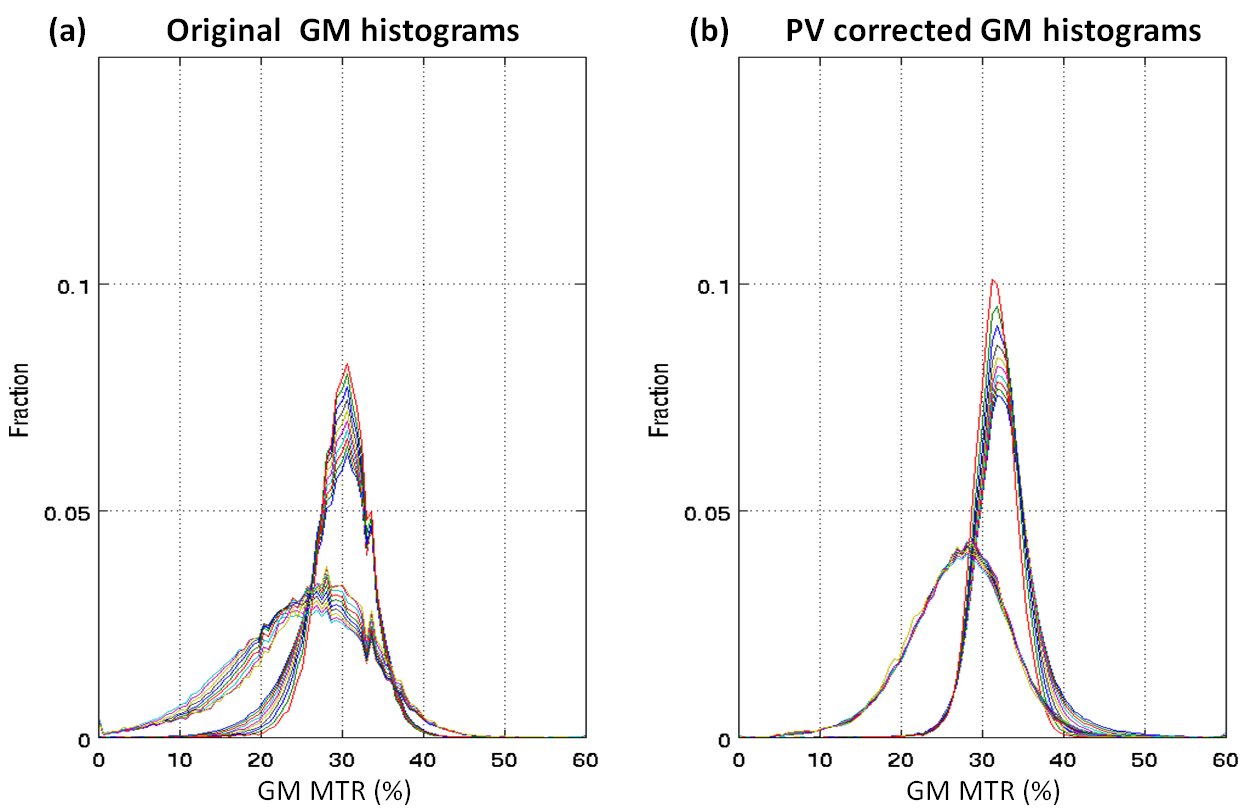
Average (standard deviation) MTR calculated over all voxels with >0.95 tissue fraction was 36.4 (2.3)% for WM and 30.7 (3.3)% respectively for WM and GM of the healthy subject; MTR was 36.1 (3.9)% and 27.8 (7.7)% for patient WM and GM. Measured and PV corrected plots for different PV fraction bins are shown in Figure 1. Measured MTR maps are shown in Figure 2 together with pvGM fraction and estimated tissue specific MTR_ pvcGM and MTR_ pvcWM maps. Figure 3 and 4 shows respectively GM and WM histograms of patient and control, before (a) and after (b) PV correction, using different colours for different PV-fraction thresholds.Discussion and Conclusions
The original MTR maps display an approximately linear dependence on PV-fraction for WM, due to the contamination with CSF with extremely low MTR values. The curves for GM are not quite as linear. This is probably due to the contrasting effect of WM contamination (causing an apparent MTR increase) and CSF contamination (causing an apparent MTR decrease). The PV corrected tissue specific MTR values from all 3 kernels used show a much lower dependence on PV-fraction demonstrating a substantial correction of PV effects, especially for PV fractions above 0.7-0.8 (typical threshold used).From Figure 3, 4 it is obvious how the histogram narrow and the PV-threshold dependence is much reduced.
Using the simple PV correction proposed the MTR histograms obtained display a much lower dependnce on PV threshold. This may help in discriminating subtle pathologies. Further work will include testing this methodology in a cohort of MS patients.
Acknowledgements
This work was supported by the National Institute for Health Research University College London Hospitals Biomedical Research Centre. DLT is supported by the UCL Leonard Wolfson Experimental Neurology Centre (PR/ylr/18575).References
No reference found.Figures