2415
Bias in Aqueductal Cerebrospinal Fluid Flow Quantification Obtained using 2D PC-MRI1Barrow Neurological Institute, Phoenix, AZ, United States, 2School of Biological Health and Systems Engineering, Arizona State University, Tempe, AZ, United States
Synopsis
This focus of this work was to determine the extent of RF saturation induced bias in cerebrospinal fluid flow quantification using 2D PCMRI. The velocity distribution within a flow region inherently biases the average estimate per voxel towards faster spins in that voxel. This effect was studied through variations in flip angle. The results indicated that higher flip angles would introduce more bias in the flow estimates, which could be a possible reason for the lack of consensus concerning the use of PCMRI in determining patient responsiveness to surgical interventions in NPH studies.
Introduction
Accuracy of phase contrast (PC) based quantitative flow measurements is an important factor when studying flow dynamics in cerebrovascular disorders such as normal pressure hydrocephalus (NPH)1,2. There is established research quantifying bias in flow estimates due to effects from resolution, partial volume and intra-voxel flow dephasing3,4,5. However, RF saturation effects on velocity estimates has not been studied to our knowledge. Flow regions may encounter varying amounts of RF pulses due to the velocity distribution of spins. The slower moving spins will be saturated to a greater extent than the faster spins in any given voxel, inducing changes to the average velocity estimate of the voxel from this inherent signal weighting. The focus of this study was to determine if RF saturation introduced a significant bias in velocity estimates for 2D PC-MRI of cerebrospinal fluid (CSF) flow in the aqueduct.Methods
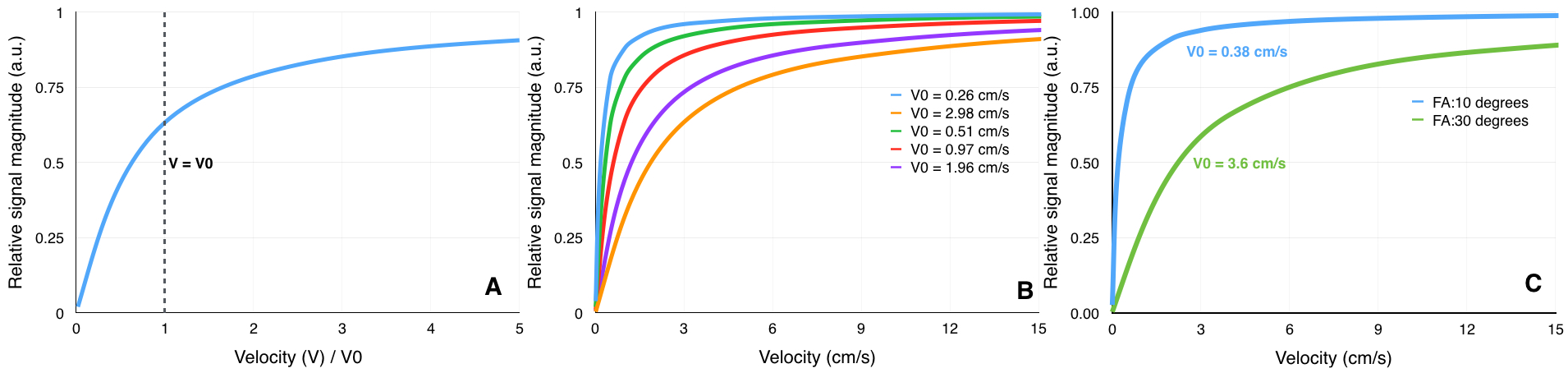
The relative signal magnitude as a function of velocity can be modeled as described in Eq. [1].
$$S=\int_{voxel} \frac{1-e^{-V_0/v}}{V_0/v} e^{\frac{-i \pi v}{V_{enc}}} dv,\;\;\;\;\;[1]$$
$$V_0=\frac{\Delta z}{TA},\;\;\;\;\;[2]$$
where S denotes signal magnitude, $$$\Delta z$$$ slice thickness, and TA the time constant describing the rate at which magnetization is removed from the system by RF pulses6, and is related to flip angle (α), and recovery time (TR) as shown in Eq. [3].
$$cos(\alpha)=e^{\frac{-TR}{TA}}.\;\;\;\;\;[3]$$
An example of the integrand ratio in Eq. [1] for relative signal magnitude was calculated as a function of velocity for flip angle (FA) variation of 100 and 300 (TR=20 ms and $$$\Delta z$$$=5 mm). Figure 1B shows example $$$V_0$$$ values calculated from referenced literature7-11. Phantom Experiments: A flow phantom was used with 2D PC-MRI (0.5x0.5mm in-plane resolution, Venc=8cm/s, $$$\Delta z$$$=5mm), to obtain data using FA =100 and 300. In vivo Experiments: Four volunteers were scanned (6 repeated measures per volunteer) using 2D spiral cardiac gated PC-MRI (0.6 x 0.6 mm in-plane resolution, Venc=12cm/s, $$$\Delta z$$$=5m). FA was varied between 100 and 300. Data Analysis: A paired t test was performed on the flow phantom data to identify regions with significant changes in velocity estimates, due to FA variation. The aqueduct in the in vivo data was segmented using thresholding of the magnitude images. Velocity difference maps were obtained by subtracting FA=10 estimates from FA=30 estimates. The spatial and temporal components of the velocity gradient maps were computed for each cardiac phase. Linear regression analysis was performed to determine correlation between bias and the spatiotemporal velocity gradient. The implementation and analysis were performed using GPI12.
Results
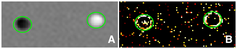
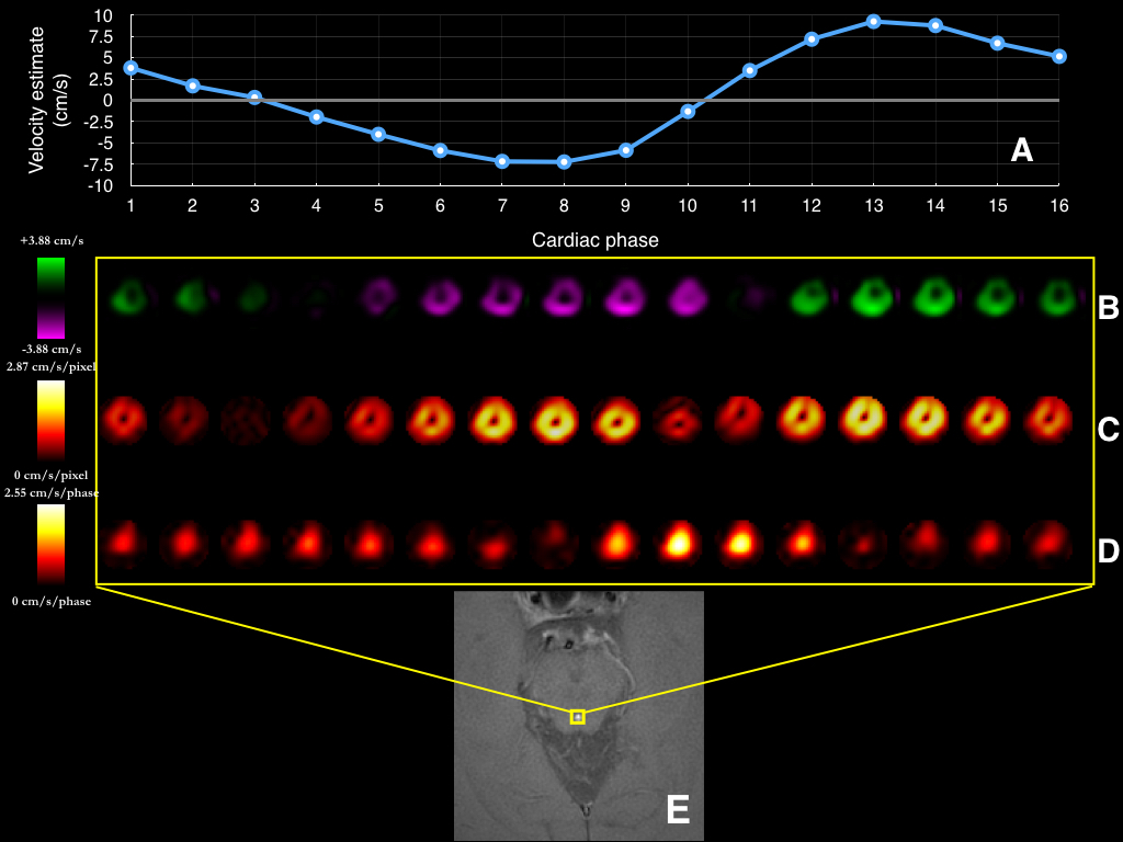
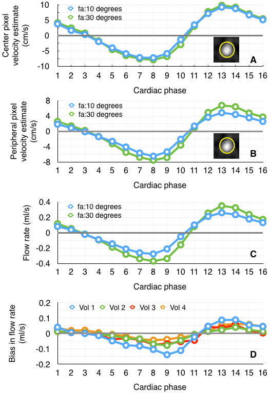
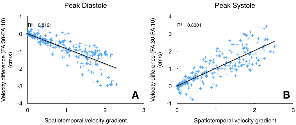
Figure 1 shows variations in relative signal magnitude as a function of velocity estimates. The results from the phantom and in vivo data are shown in Fig.2, and Fig.3 respectively. The p-value maps of Fig. 2 indicate regions with significant change in velocity estimates (p<0.05). Signed velocity difference maps obtained for FA variation in the case of aqueductal flow in vivo are shown in Fig. 3B, along with the spatial and temporal components of the velocity gradient (Fig. 3C & 3D respectively). The region of interest (ROI) is highlighted in Fig. 3E. The velocity and flow estimates obtained are compared in Fig.4. Velocity estimates are shown for a single pixel at the flow region center(Fig.4A) and periphery (Fig.4B). Figure 5 shows the correlation between the bias and spatiotemporal velocity gradient, for cardiac phases corresponding to peak diastole and peak systole.Discussion
P-value maps generated for the flow phantom, indicated that regions with greatest variation in flow (vessel periphery) incurred greater bias. In vivo, spatial and temporal variations in velocity estimates are observed due to pulsatile nature of CSF flow. Signed velocity difference maps from in vivo data, indicated higher bias at the aqueduct periphery. This effect was pronounced during cardiac phases with high spatial and low temporal velocity gradient. A linear fit between bias and spatiotemporal velocity gradient at peak diastole and systole indicated that approximately 80% of bias due to FA variations could be explained by variations in the spatiotemporal velocity gradient. This observation is consistent with the expectation that RF saturation effects are more prominent at the vessel periphery, where the velocity gradient is higher than the vessel center. This observation was also supported by the bias in single pixel velocity estimates being smaller for the center pixel than pixel at the vessel periphery. The bias was cumulative when computing flow rates from velocity estimates.Conclusion
Flip angle variation produced a noticeable bias in CSF flow quantitation in the aqueduct, and could be a contributing factor for the lack of consensus in using 2D PC-MRI for evaluating surgical intervention benefits in NPH patients.Acknowledgements
This work was funded in part by Philips Healthcare.References
1. Forner Giner J, Sanz-Requena R, Flórez N et al. Quantitative phase-contrast MRI study of cerebrospinal fluid flow: a method for identifying patients with normal-pressure hydrocephalus. Neurologia. 2014 Mar;29(2):68-75.
2. Luetmer PH, Huston J, Friedman JA et al. Measurement of cerebrospinal fluid flow at the cerebral aqueduct by use of phase-contrast magnetic resonance imaging: technique validation and utility in diagnosing idiopathic normal pressure hydrocephalus. Neurosurgery. 2002 Mar;50(3):534-43; discussion 543-4.
3. Tang C, Blatter DD, Parker DL. Accuracy of phase-contrast flow measurements in the presence of partial-volume effects. J Magn Reson Imaging. 1993;3:377–385.
4. Ku DN, Biancheri CL, Pettigrew RI et al. Evaluation of magnetic resonance velocimetry for steady flow. J Biomech Eng. 1990;112:464–472.
5. Papaharilaou Y, Doorly DJ, Sherwin SJ. Assessing the accuracy of two-dimensional phase-contrast MRI measurements of complex unsteady flows. J Magn Reson Imaging. 2001 Dec;14(6):714-23.
6. Pipe JG, Robison RK. Simplified Signal Equations for Spoiled Gradient Echo MRI. Proc. Intl. Soc. Mag. Reson. Med. 2010: 3114.
7. Beggs CB, Magnano C, Shepherd SJ et al. Aqueductal cerebrospinal fluid pulsatility in healthy individuals is affected by impaired cerebral venous outflow. J Magn Reson Imaging. 2014 Nov;40(5):1215-22. doi: 10.1002/jmri.24468. Epub 2013 Nov 8.
8. Algin O, Hakyemez B, Parlak M. The efficiency of PC-MRI in diagnosis of normal pressure hydrocephalus and prediction of shunt response. Acad Radiol. 2010 Feb;17(2):181-7.
9. Jaeger M, Khoo AK, Conforti DA et al. Relationship between intracranial pressure and phase contrast cine MRI derived measures of intracranial pulsations in idiopathic normal pressure hydrocephalus. J Clin Neurosci. 2016 Nov;33:169-172.
10. Kapsalaki E, Svolos P, Tsougos I et al. Quantification of normal CSF flow through the aqueduct using PC-cine MRI at 3T. Acta Neurochir Suppl. 2012;113:39-42.
11. Weinzierl MR, Krings T, Ocklenburg C et al. Value of cine phase contrast magnetic resonance imaging to predict obstructive hydrocephalus. J Neurol Surg A Cent Eur Neurosurg. 2012 Jan;73(1):18-24.
12. Zwart NR, Pipe JG. Graphical programming interface: A development environment for MRI methods. Magn Reson Med. 2015 Nov;74(5):1449-60.
Figures