1988
Towards Eliminating Magnetization Transfer (MT) Effect on CEST Quantification Using MR Fingerprinting: Simulations1Department of Engineering Physics, Tsinghua University, Beijing, People's Republic of China, 2Key Laboratory of Particle and Radiation Imaging, Ministry of Education, Beijing, People's Republic of China, 3Biomedical Imaging Research Institute, Cedars-Sinai Medical Center, Los Angeles, CA, United States, 4Department of Bioengineering, University of California Los Angeles, Los Angeles, CA, United States, 5Department of Imaging, Cedars-Sinai Medical Center, Los Angeles, CA, United States
Synopsis
In this work, a new quantitative chemical exchange saturation transfer (q-CEST) method based on MR fingerprinting is developed to eliminate the influence of MT effect. Signal evolutions are generated by using a series of hard saturation pulses with different amplitudes and durations. The dictionary is constructed using the 2-pool model. Simulation experiments based on the 3-pool model were performed, and simulation results show that good mapping accuracy was achieved even in the presence of the MT effect.
Introduction
CEST MRI is a rather complicated system with many confounding factors. Even though current methods can quantify the exchange rate and labile proton fraction ratio by eliminating the effects from T1, T2 and spillover effects, magnetization transfer (MT) effects still remain as a contamination factor in the CEST quantification.1,2,3
MR Fingerprinting (MRF) is a novel method for simultaneous multi-parametric mapping.4 One of its most important features is that it involves a pattern recognition algorithm to match the MR signal to a predefined dictionary. It is important to note that the pattern recognition process only takes into consideration the shape of the signal evolution, therefore, the signal magnitude does not affect the result.
In this study, we apply a similar idea to CEST MRI. We hypothesize that the CEST signal evolutions with and without the presence of the MT effects have the same shape, even though the magnitudes are different, allowing accurate CEST quantification.
Methods
Sequence Design
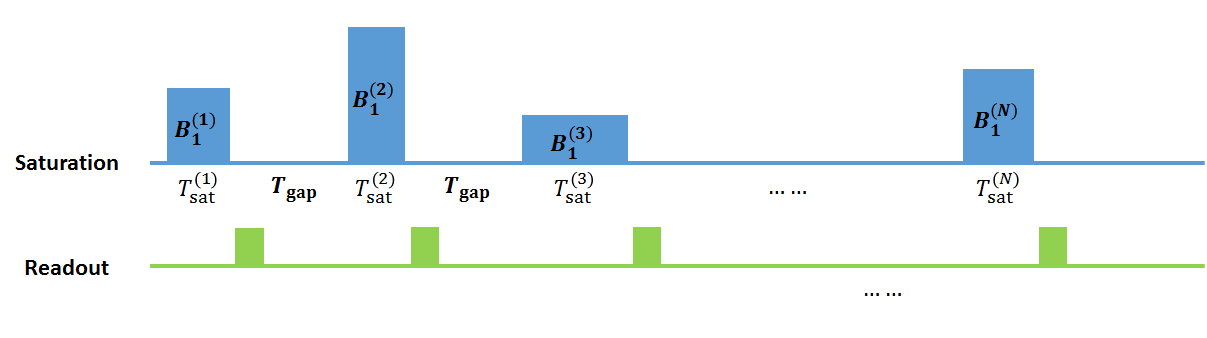
The pulse sequence used in the method is illustrated in figure 1. A number of saturation-readout units are performed one by one in a single scan. Hard saturation pulses with different amplitudes ($$$B_1^{(i)}$$$) and durations ($$$T_{sat}^{(i)}$$$) are used in different units. Before each saturation, the transverse magnetization is dephased. $$$B_1$$$ ranges from 0.3-2.7 μT, $$$T_\text{sat}$$$ ranges from 0.8-2.0 sec, $$$T_\text{gap}=300\text{ms}$$$, $$$\alpha=45^\circ$$$, and $$$N = 50$$$.
The sequence is performed twice, at saturation frequency of $$$+\Delta\omega$$$ and $$$-\Delta\omega$$$, to get the 50 CESTRasym’s ($$$\text{CESTR}_\text{asym}^{(i)}=\frac{S^{(i)}(-\Delta\omega)-S^{(i)}(\Delta\omega)}{S_0}$$$), which is used as the signal evolution.
Dictionary
The dictionary is built based on the 2-pool Bloch-McConnell Equations with different exchange rates ($$$k_\text{sw}$$$) ranging from 10-500 s-1), in which T1 and T2 values of the water pool ($$$T_1^\text{w}$$$ and $$$T_2^\text{w}$$$) are determined by preceding mapping methods, while the T1 and T2 values of the solute pool ($$$T_1^\text{s}$$$ and $$$T_2^\text{s}$$$) and the labile proton ratio ($$$f_\text{r}$$$) are fixed ($$$T_1^\text{s} = 1000\text{ms}$$$, $$$T_2^\text{s} = 20\text{ms}$$$, $$$f_\text{r} = \text{1:500}$$$). Each entry vector of the dictionary is the CESTRasym’s for a particular exchange rate. Although the MT effect would reduce the amplitude of readout signal, the subtraction of $$$S^{(i)}(-\Delta\omega)-S^{(i)}(\Delta\omega)$$$ cancels such effect in part. Furthermore, the matching method of normalized dot product is used, so that only the shape of the signal evolution affects the matching accuracy.
Simulations
We performed the numerical simulations in MATLAB for creatine protons, with $$$\Delta\omega = 2.0\text{ppm}$$$. The signal evolutions were simulated using the 3-pool Bloch-McConnell Equations.5 In the simulation, the T1 and T2 values of the MT pool were fixed (1000ms and 0 respectively), the exchange rate of MT effect was set to be 100s-1 and Rrfb, the parameter used to represent the RF absorption profile for MT pool, was set to be 1. Set $$$B_0 = 3.0\text{T}$$$. The signal evolutions from 1000 samples were simulated with different $$$T_1^\text{w}$$$(1000-2000ms), $$$T_2^\text{w}$$$(100-200ms), $$$T_1^\text{s}$$$(800-1200ms), $$$T_2^\text{s}$$$(10-50ms), $$$k_\text{sw}$$$(100-500s-1) and $$$f_\text{r}$$$(1:1000-1:500). Noises were added to simulate different SNRs. Then the ksw and pH value were determined using the dictionary matching method, where the pH value is calculated using the formula $$$k_\text{sw} = k_0 + k_b \times 10^{\text{pH}-\text{pkw}}$$$, with $$$k_0=7.0, k_b=1.4, \text{pkw}=4.8$$$.6 The mean relative error for ksw mapping and mean error of pH mapping were calculated, i.e. $$$\sigma(k_\text{sw}) = \text{mean}\left|{\frac{k_\text{sw}-k_\text{sw,real}}{k_\text{sw,real}}} \right|$$$, $$$\Delta\text{pH} = \text{mean}\left|\text{pH}-\text{pH}_\text{real}\right|$$$.
Results
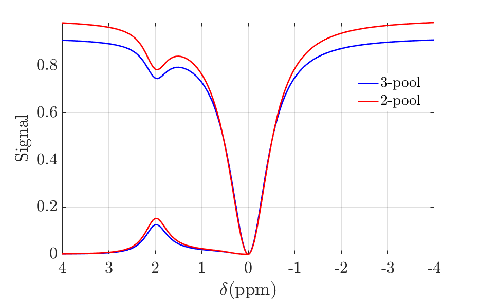
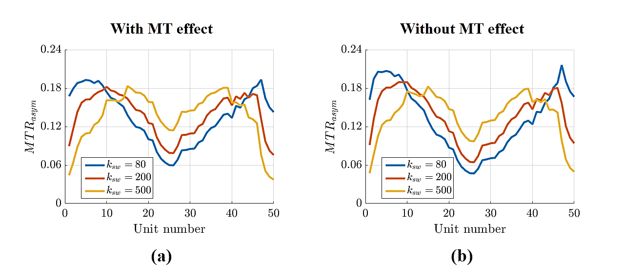
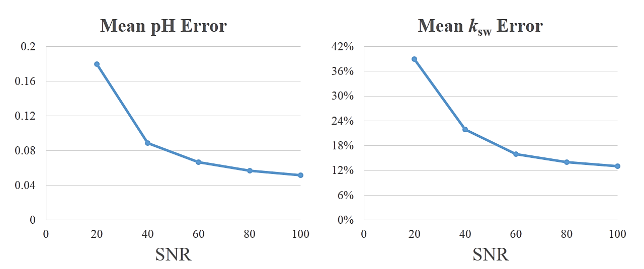
Figure 2 shows the simulated Z-spectrum of 2-pool and 3-pool model, in which the MT effect can be seen clearly. Figure 3 shows the normalized signal evolutions of ksw = 80, 200 and 500 (i.e. pH = 6.5, 6.9 and 7.4) with MT effect (in fig. 3(a)) and without MT effect (in fig. 3(b)), and all other parameters were fixed. It can be seen in fig. 3 that the shapes of the signal evolutions remain largely the same in the existence of the MT effect. Figure 4 shows that the mapping error decreases with higher SNR, achieving 0.1 or less pH error when SNR is larger than 40. All the figures were generated with simulation.Conclusion
In this work, we simulated a new MR fingerprinting CEST quantification method to eliminate the contamination from the MT effects.It allows more accurate pH measurement. This method needs to be validated with imaging experiments.Acknowledgements
No acknowledgement found.References
1. Sun, Phillip Zhe, et al. "Simultaneous experimental determination of labile proton fraction ratio and exchange rate with irradiation radio frequency power-dependent quantitative CEST MRI analysis." Contrast media & molecular imaging 8.3 (2013): 246-251.
2. Meissner, Jan-Eric, et al. "Quantitative pulsed CEST-MRI using Ω-plots." NMR in Biomedicine 28.10 (2015): 1196-1208.
3. Zhou, Zhengwei, et al. "Quantitative chemical exchange saturation transfer MRI of intervertebral disc in a porcine model." Magnetic Resonance in Medicine (2016).
4. Ma, Dan, et al. "Magnetic resonance fingerprinting." Nature 495.7440 (2013): 187-192.
5. Desmond, Kimberly L., and Greg J. Stanisz. "Understanding quantitative pulsed CEST in the presence of MT." Magnetic resonance in medicine 67.4 (2012): 979-990.
6. Wu, Renhua, et al. "Quantitative description of radiofrequency (RF) power-based ratiometric chemical exchange saturation transfer (CEST) pH imaging." NMR in Biomedicine 28.5(2015):555–565.
Figures