1963
Accuracy of magnetic resonance based susceptibility measurements1Precision Measurement Laboratory, NIST, Boulder, CO, United States, 2Department of Physics, University of Colorado Boulder, Boulder, CO, United States
Synopsis
We examined the accuracy of MR-based susceptibility quantification relative to conventional measurements in preparation of making a standard susceptibility phantom. SQUID magnetometry of tissue mimics provides absolute accuracy of approximately 100 ppb while MR-based techniques give relative accuracy of 10 ppb.
Introduction
Quantitative Susceptibility Mapping (QSM)1 is increasingly used instead of qualitative techniques, such as susceptibility weighted imaging,2 to map neural diseases,3-5 blood oxygen content,6 and iron overload in the heart and liver.7 Creating standard measurement protocols and a NIST-verified susceptibility phantom would help ensure site-to-site comparability of data and allow wide-spread and reliable use of QSM in clinical applications. SQUID (superconducting quantum interference device) magnetometry measurements of excised tissue susceptibility are inaccurate due to water loss, blood oxidation, and volume changes. In-vivo MRI susceptibility measurements, if done properly, may become the gold standard for tissue susceptibility quantification. The first step is to verify the accuracy of MRI susceptibility measurements relative to other traditional methods.8Methods
Magnetic moment measurements were made in a SQUID magnetometer using NIST SRM #2852 for calibration. Gradient echo phase images of susceptibility phantoms were obtained in a pre-clinical scanner. Post-processing of the phase images included phase unwrapping and long wavelength background subtraction. The phase vs echo time was fit to a line to obtain the susceptibility using the long cylinder approximation (Eq.1): $$δB_L=\frac{ΔχB_0}{6}(3cos^2θ-1)$$
Results
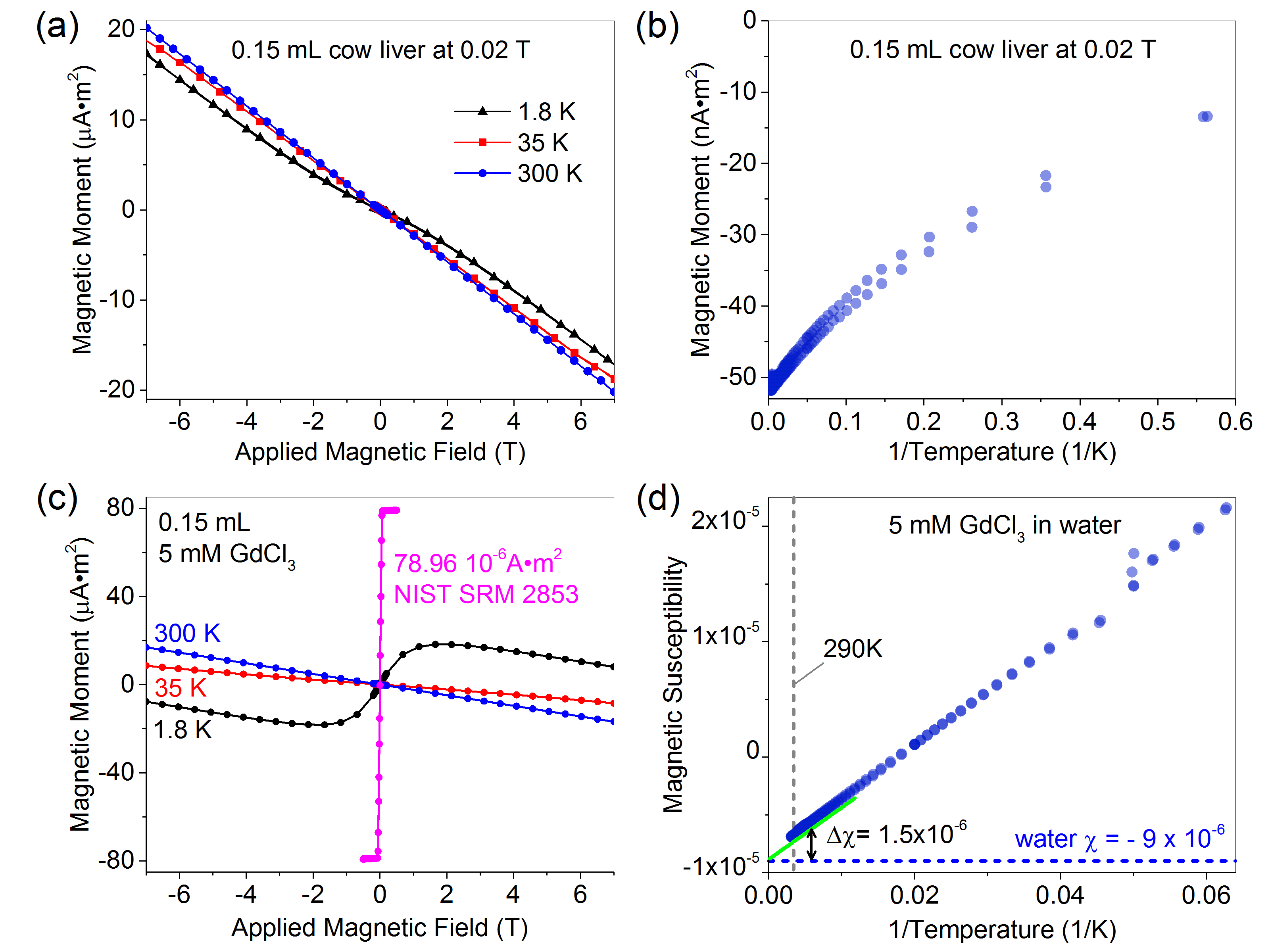
Tissue is predominantly diamagnetic at body temperature 310K as shown in Fig.1a, which plots magnetic moment vs. field of cow liver. The magnetic susceptibility is dominated by diamagnetic water (-9.05*10-6) and fat (~-10.0*10-6).9 Complex magnetic structure of tissue is seen at lower temperatures. Fig.1a shows a decrease in the diamagnetic (negative) slope as the temperature decreases indicative of a paramagnetic component. Deviations in linearity due to paramagnetic and ferrimagnetic components exist at low temperature (1.8K). A ferrimagnetic characteristic is seen in the moment vs. inverse temperature plot of Fig.1b. With only a paramagnetic component, the data would be linear. For liver, the paramagnetic and ferrimagnetic components are predominantly due to deoxyhemoglobin and iron oxide deposits (ferritin). To mimic the susceptibility properties of tissue, one can use paramagnetic salt solutions. Fig.1d shows schematically how water, with a diamagnetic susceptibility of minimal temperature-dependence and a paramagnetic component can approximate the magnetic properties of tissue. We present data from GdCl3 solutions, whose magnetic properties are shown in Fig.1c,d for a 5.0mM solution in deionized water.
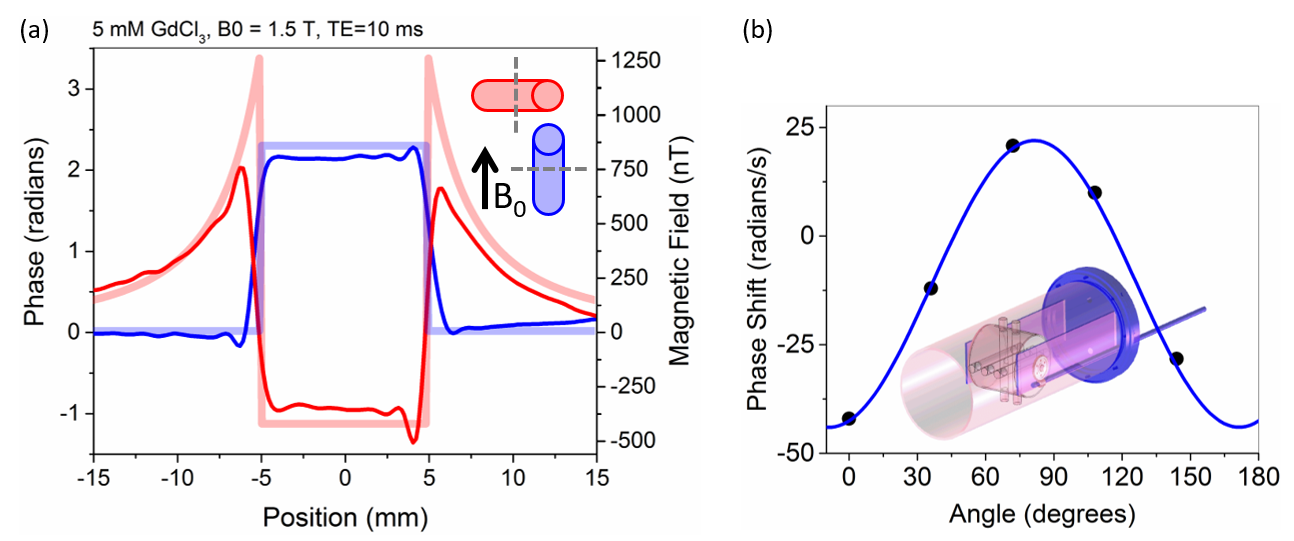
To more precisely verify orientation dependence, a rotating phantom was constructed with continuously rotating 80mm vials (schematic shown in Fig.2b inset). Four 80mm vials filled with 1.0mM and 5.0mM GdCl3 solutions were scanned. A rod extended out of the scanner from the internal gears; each revolution corresponded to 19-degree mechanical rotation of phantom insert. Phase shifts across each water-surrounded vial were collected as a function of angle, Fig.2b. Results were fit using Eq.1 yielding Δχ= (3.24 ± 0.05)*10-7 for the 1.0mM solution.
Discussion: Other Sources of Error
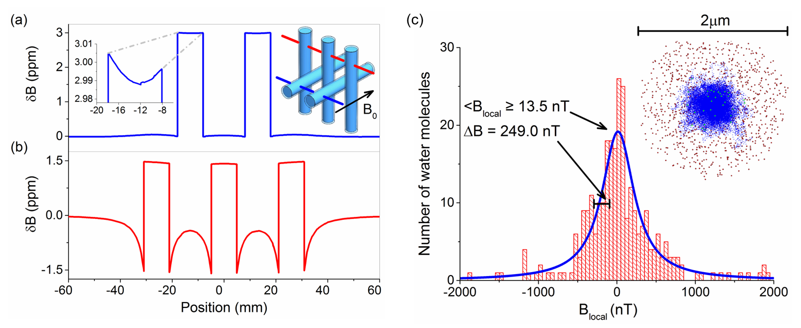
Finite element simulations were used to compute the macroscopic field of the phantom in Fig.2b inset. The vials were filled with a solution with a magnetic susceptibility of 3.0*10-6 relative to surrounding water to simulate our 5.0mM GdCl3 experiment. Fig.3a,b show field distortions when the B0 field is parallel and perpendicular to the vial axes, respectively. The field profiles within the vials are not constant, as predicted by the simple models, due to the fields from neighboring vials, the finite length of the vials, and the phantom structure.
One main approximation in MR-based susceptibility measurements is to assume that the local field is the macroscopic field minus the Lorentz field and the local microscopic fields average to zero. To determine the local field, precise microscopic calculations are needed. As a simple test, Monte Carlo calculations were performed; 2.5*106 Gd3+ spins were randomly distributed in 2μm diameter sphere filled with 300 diffusing water molecules. The fields sensed by the water molecules after a time of 0.15 ms are plotted in Fig.4c. The Gd density corresponds to 1mM concentration and a susceptibility of 3.2*10-7. The microscopic field calculated from the simulation is 13.5nT, which is much smaller than the Lorentz field BL= 320nT. The simulation supports the assumption that the microscopic fields due to neighboring spins average to zero and the local field approximation is valid. For tissues, which may have more complex local geometry, this local field assumption may not be valid.
Conclusion
Relative phase shifts and local induced magnetic fields can be measured very precisely with MRI. The relative susceptibilities can be accurately determined from these field shifts for simple geometries and agree with primary measurements of susceptibility where standards exist. More suitable primary standards, however, will be required to validate MRI susceptibility measurements in complex geometries. More extensive investigation into how the local field depends on microscopic tissue geometry is required to determine the accuracy of local field models.Acknowledgements
No acknowledgement found.References
1. Wang Y and Liu T. Quantitative susceptibility mapping (QSM): Decoding MRI data for a tissue magnetic biomarker. Magn Reson Med. 2015;73(1):82-1012.
2. Haacke E M, Mittal S, Wu Z, Neelavalli J, and Cheng Y C. Susceptibility-weighted imaging: technical aspects and clinical applications, part 1. AJNR Am J Neuroradiol. 2009;30(1):19-303.
3.Jensen J H, Szulc K, Hu C, Ramani A, Lu H, Xuan L, Falangola M F, Chandra R, Knopp E A, Schenck J, Zimmerman E A, and Helpern J A. Magnetic field correlation as a measure of iron-generated magnetic field inhomogeneities in the brain. Magn Reson Med. 2009;61(2):481-4854.
4. Shmueli K, de Zwart J A, van Gelderen P, Li T Q, Dodd S J, and Duyn J H. Magnetic susceptibility mapping of brain tissue in vivo using MRI phase data. Magn Reson Med. 2009;62(6):1510-15225.
5. Tan H, Liu T, Wu Y, Thacker J, Shenkar R, Mikati A G, Shi C, Dykstra C, Wang Y, Prasad P V, Edelman R R, and Awad I A. Evaluation of iron content in human cerebral cavernous malformation using quantitative susceptibility mapping. Invest Radiol. 2014;49(7):498-5046.
6. Haacke E M, Prabhakaran K, Elangovan I R, Wu Z, and Neelavalli J. Oxygen Saturation: Quantification, in Susceptibility Weighted Imaging in MRI: Basic Concepts and Clinical Applications. (eds E. M. Haacke and J. R. Reichenbach). John Wiley & Sons, Inc. 2011;517-528.
7. Sharma S D, Hernando D, Horng D E, and Reeder S B. Quantitative susceptibility mapping in the abdomen as an imaging biomarker of hepatic iron overload. Magnetic Resonance in Medicine. 2015;74(3):673-6838.
8. Erdevig H E, Russek S E, Carnicka S, Keenan K E, Stupic K F. Accuracy of magnetic resonance based susceptibility measurements. Accepted for publication in AIP Advances. 2017.
9. Schenck J F. The role of magnetic susceptibility in magnetic resonance imaging: MRI magnetic compatibility of the first and second kinds. Medical Physics. 1996;23(6):815-850.
Figures