Purpose

Quantitative susceptibility mapping (QSM) provides novel insights into tissue composition, iron accumulation and myelination^1–3. Susceptibility effects scale with the static magnetic field and as such QSM profits from the availability of ultra-high field scanners. However, one challenge at ultra-high field is the channel combination of phase data from phased array receive coils. It is possible to avoid the combination of signal phase across channels as a first step by calculating QSMs for each channel separately. These can then be combined using an arithmetic mean across channels. However, this requires each channel to have adequate coverage of the object and sufficient SNR to allow an estimation of the background field and the solution of the QSM inverse problem. This method has been shown to yield susceptibility maps without obvious artifacts⁴, but it has not yet been tested how this method compares to a reference-based approach - COMbining Phase data using a Short Echo-time Reference scan (COMPOSER) – which can approximate the true phase offsets⁵.

Methods

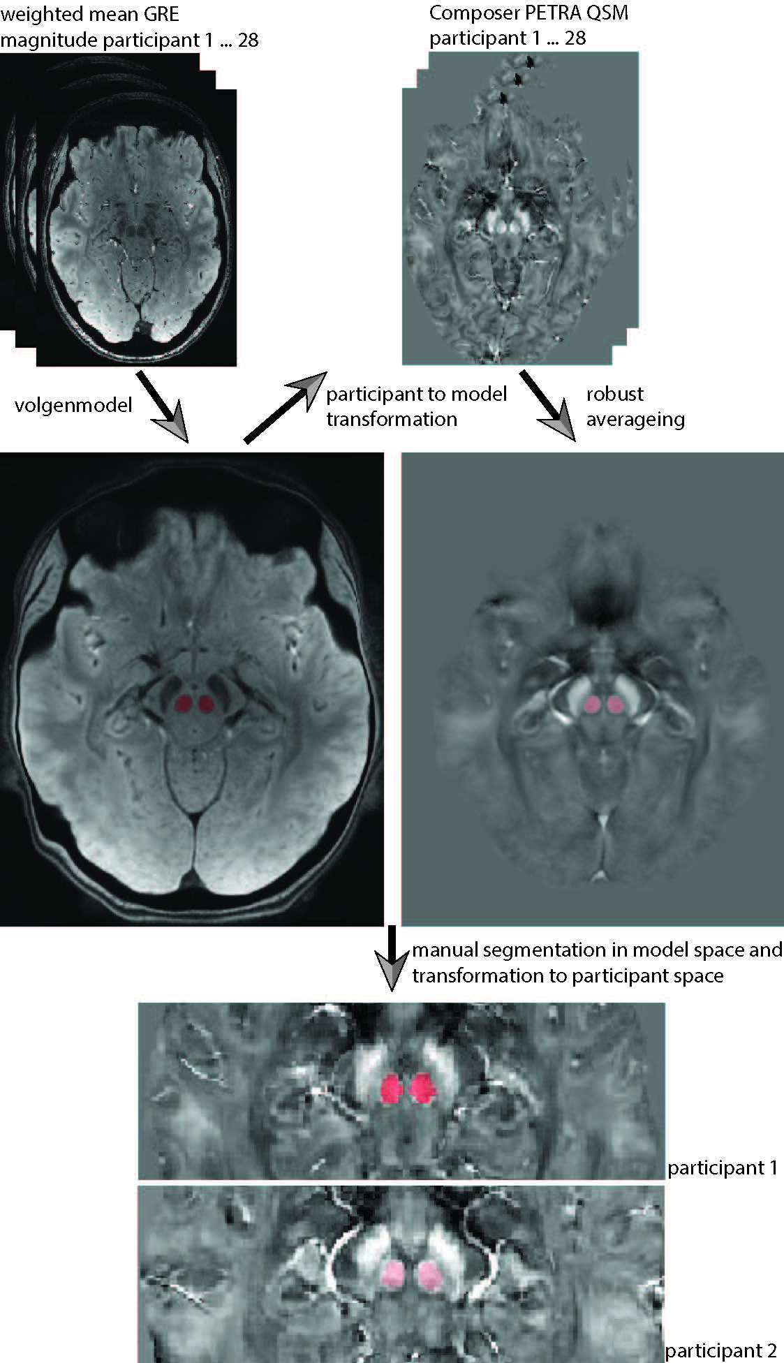
After approval by the local human ethics committee and written informed consent, 28 participants (21-34 years of age, 14 males) were investigated on a 7T whole-body research scanner (Siemens Healthcare, Erlangen, Germany) and a 32-channel head coil (Nova Medical, Wilmington, USA). We acquired a multiple-echo gradient-recalled echo (GRE) 3D whole-brain dataset: TR=25ms, TE=4.4,7.25,10.2,13.25,16.4,19.65,23ms, flip angle=13 degree, FOV=210x181.5x120mm³, matrix=280x242x160, GRAPPA = 2, TA=7.9min. For the reference scans both, a GRE with 3 echoes (TR=8ms, TE=1.02,3.06,6.12ms, flip angle=5 degree, FOV=245x245x182mm³, matrix=70x70x52, GRAPPA = 1, TA=24s), and a prototype ultra-short-TE sequence PETRA⁶, were acquired (TR=1.99ms, TE=0.07ms, flip angle=2 degree, FOV=288x288x288mm³, matrix=288x288x288, GRAPPA=1, TA=2min). Susceptibility maps were calculated using total generalized variation (TGV)⁷. The single-channel approach processed each coil channel individually and the final susceptibility maps were calculated by computing the mean across all channels. For COMPOSER, the short-TE GRE sequence (2 echoes: 1.02, 3.06ms) and the ultra-short-TE PETRA sequence (1 echo: 0.07ms) were both used to attempt to correct the phase offsets and combine the phase data. An atlas-based segmentation⁸ was used to extract susceptibility values of all subjects from manually segmented regions of interest (Figure 1).

Results & Discussion

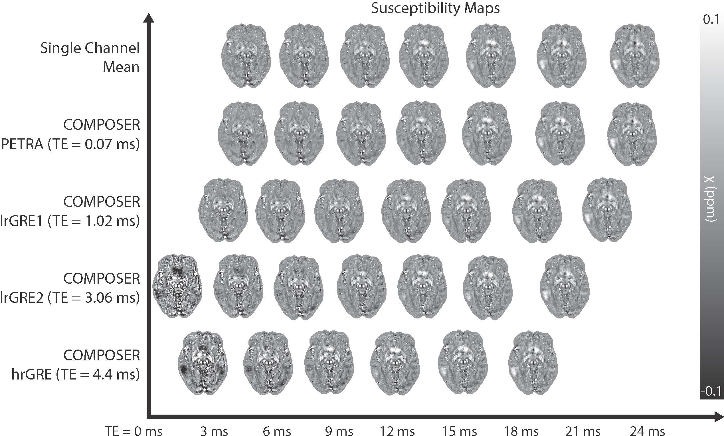
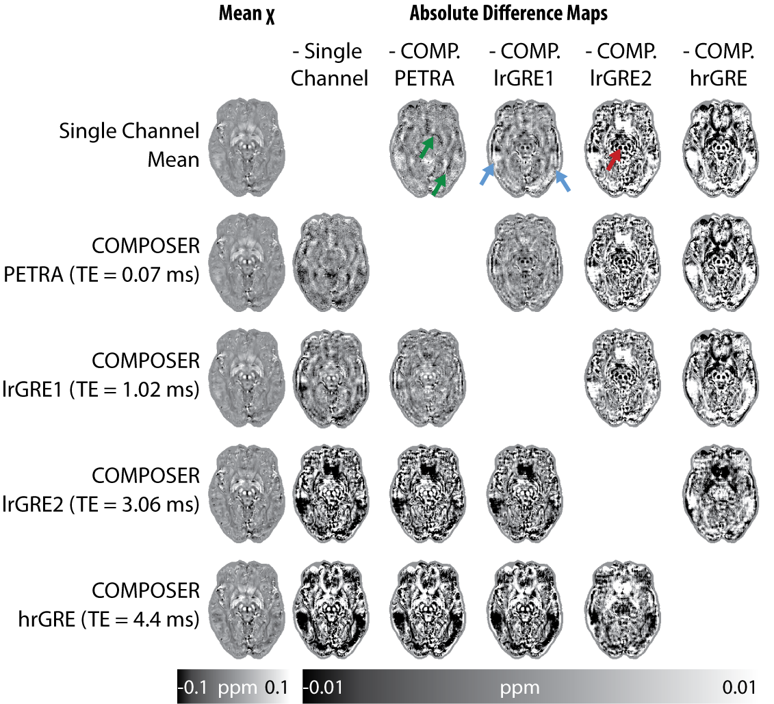
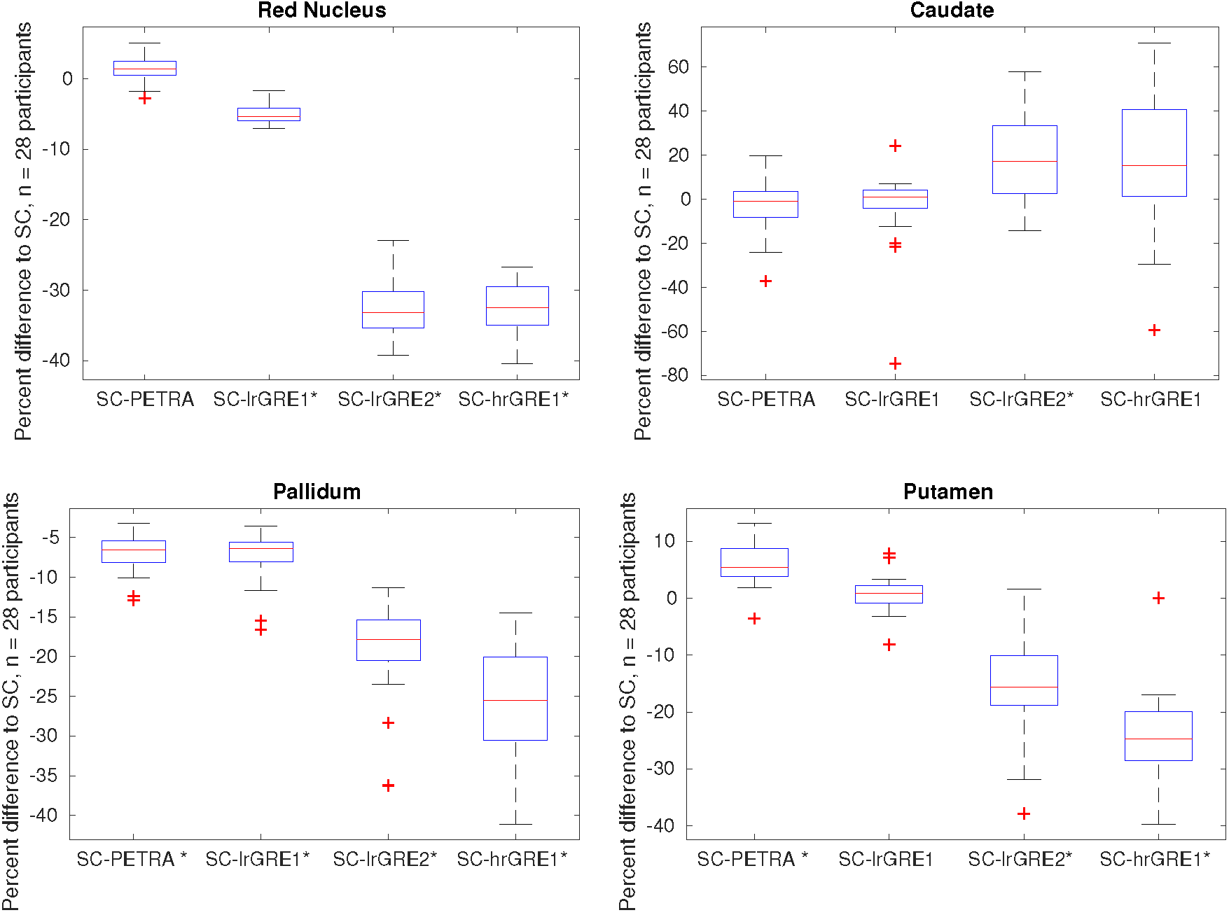
Figure 2 shows the susceptibility maps computed based on the combined phase data and the single-channel approach in the top row, most of which appear strikingly similar. Therefore, all pipelines were also compared by calculating absolute-difference susceptibility maps shown in Figure 3. The PETRA reference scan and the first echo of the low resolution GRE (lrGRE1) show similar results except for Gibbs ringing artifacts when using the low resolution reference scan, which is more clearly seen in cortical regions (blue arrows) in Figure 3. This is due to the fact that only a low spatial resolution is achievable with a short echo-time. When the second echo of the low resolution GRE (lrGRE2) is used as a reference scan, one can see that the first combined echo shows a very low contrast (see Figure 2). Further, these reference scans also show a difference in subcortical regions like the red nucleus in this participant (red arrow, Figure 3). As expected, the high resolution GRE reference scan introduces slightly more noise in the susceptibility maps due to an SNR decrease, but does not suffer from the Gibbs ringing artifacts in comparison to the low resolution reference scans. However, it shows a different gray/white matter contrast, which implies a reference scan phase evolution difference between these regions, which in this case, increases the contrast. Finally, in Figure 3, the comparison between the single-channel approach and the PETRA reference scan shows that there is a structured difference pattern (green arrows), which was not apparent in Figure 2. Assessment of computed susceptibility values in specific brain regions for all 28 subjects as a function of echo time are shown in Figure 4. A marked deviation between pipelines exists for early echoes and reduces at later echo times. The relative difference between all COMPOSER combinations and the single-channel method is shown in Figure 5. Statistically significant differences (FWER p < 0.001, 16 tests, Bonferroni corrected p < 0.0000625) between the single-channel method and the COMPOSER combinations are marked with an asterisk.

Conclusions

Our comparison of the various coil combination approaches in the tested QSM pipeline implies that deficiencies in reference scans can bias QSM results. An ultra-short echo time reference scan reduces this bias, and the single-channel approach provides a robust method and similar results.

Acknowledgements

SB acknowledges funding from UQ Postdoctoral Research Fellowship grant and support via an NVIDIA hardware grant. MB acknowledges funding from ARC Future Fellowship grant FT140100865. The authors acknowledge the facilities of the National Imaging Facility at the Centre for Advanced Imaging, University of Queensland and the scientific support of Siemens Ltd, Bowen Hills, Australia.