Synopsis

We investigate the computational aspects of the prior term in the field-to-susceptibility inversion problem for QSM. Providing a spatially continuous formulation of the problem, we analyze 1) its Euler-Lagrange equation that appears degeneracy and 2) the Gauss-Newton conjugate gradient (GNCG) algorithm that employs numerical conditioning. We propose a primal-dual (PD) formulation that avoids such degeneracy and use the Chambolle-Pock algorithm to solve this alternative formulation; thus numerical conditioning is not required. The two methods were tested and validated on numerical/gadolinium phantoms and ex-vivo/in-vivo MRI data. The PD formulation with the Chambolle-Pock algorithm was faster and more accurate than GNCG.

Purpose

Theory

1) Energy Functional

In a spatially continuous setting, the problem of morphology-enabled dipole inversion (MEDI) (1) can be expressed as follows:

$$ \text{Find } \hat \chi \text{ such that } \hat \chi \in \operatorname{Argmin}\left\{\chi \in BV(\Omega; \mathbb{R}): \int_\Omega |M\nabla \chi|_1 + \frac{\lambda}{2}\int_\Omega |w(d*\chi-b)|^2\right\}$$

Here, the susceptibility distribution $$$\chi:(\Omega\subset\mathbb{R}^3)\to \mathbb{R}$$$ is estimated from the measured local field $$$b:\Omega\to\mathbb{R}$$$. The space of bounded variation, $$$BV(\Omega;\mathbb{R})$$$ , allows the existence of jumps modeling sharp edges. The map $$$w:L^1\to L^1$$$ compensates for the non-uniform phase noise (SNR weighting), and the edge indicator map $$$M:[L^1]^3 \to [L^1]^3$$$ is derived from the corresponding magnitude image.

2) GNCG

GNCG assumes that $$$\chi$$$ is differential, which allows us to derive the Euler-Lagrange (EL) equation associated with the energy functional as follows:

$$ \sum_{\ell=1}^3 \frac{\partial}{\partial r_\ell}\left( \frac{M_{r_\ell(r)}\partial_{r_\ell}\chi(r)}{|M_{r_\ell(r)}\partial_{r_\ell}\chi(r)|} \right) - \lambda (w(d*))^H(w(d*\chi-b))=0, \quad \forall r=(r_1, r_2, r_3) \in int\,\Omega, $$

where $$$(w(d*))^H$$$ is the adjoint of $$$w(d*)$$$. The EL equation, however, exhibits degeneracy when $$$|M_{r_\ell(r)}\partial_{r_\ell}\chi(r)|=0$$$ so that numerical conditioning is required for computational purposes: $$$|M_{r_\ell(r)}\partial_{r_\ell}\chi(r)|$$$ is replaced with $$$\sqrt{|M_{r_\ell(r)}\partial_{r_\ell}\chi(r)|^2 +\epsilon}$$$ for $$$\ell=1,2,3$$$ and $$$\epsilon>0$$$. As a consequence, this conditioning deviates from the definition of total variation, which leads to solving a slightly different objective.

3) PD

We can derive a generalized definition of anisotropic weighted total variation as follows:

$$\int_\Omega |M\nabla\chi|_1 = \sup \left\{ -\int_\Omega \chi(r)\operatorname{div}(M^H(r)\xi(r))dr : \xi \in C_c^1(\Omega;\mathbb{R}^3), ||\xi(r)||_\infty \leq 1, \forall r \in \Omega \right\}$$,

where $$$C_c^1$$$ is the set of continuously differentiable functions with compact support. $$$\xi$$$ is the so-called dual variable with the constraint of pointwise maximum norm. Note that the discontinuities are allowed in $$$\xi$$$ in the above dual formulation. Additional dualization for the data fidelity term (2) leads us to the following primal-dual formulation:

$$ \hat \chi \in \operatorname{Argmin} \left\{ \operatorname{sup} \left\{ (\xi, \nu) \in C_c^1 \times L^2 : -\int_\Omega \chi \operatorname{div}(M^H\xi) + \langle w(d*\chi-b), \nu \rangle_{L^2} - \iota_P(\xi) - \frac{1}{2\lambda} ||\nu||_2^2 \right\} \right\}$$,

where the indicator function $$$\iota(\xi)$$$ of a set $$$P\subset C_c^1$$$ is defined as $$$\iota_P(\xi)=0$$$ if $$$\xi \in P$$$, $$$+\infty$$$ otherwise. Here, the convex set $$$P=\{\xi\in C_c^1(\Omega;\mathbb{R}^3) : ||\xi(r)||_\infty \leq 1, \forall r \in \Omega\}$$$. This saddle-point problem can be solved by the Chambolle-Pock algorithm (3). Note that GNCG now can be viewed as the primal approach.

Methods

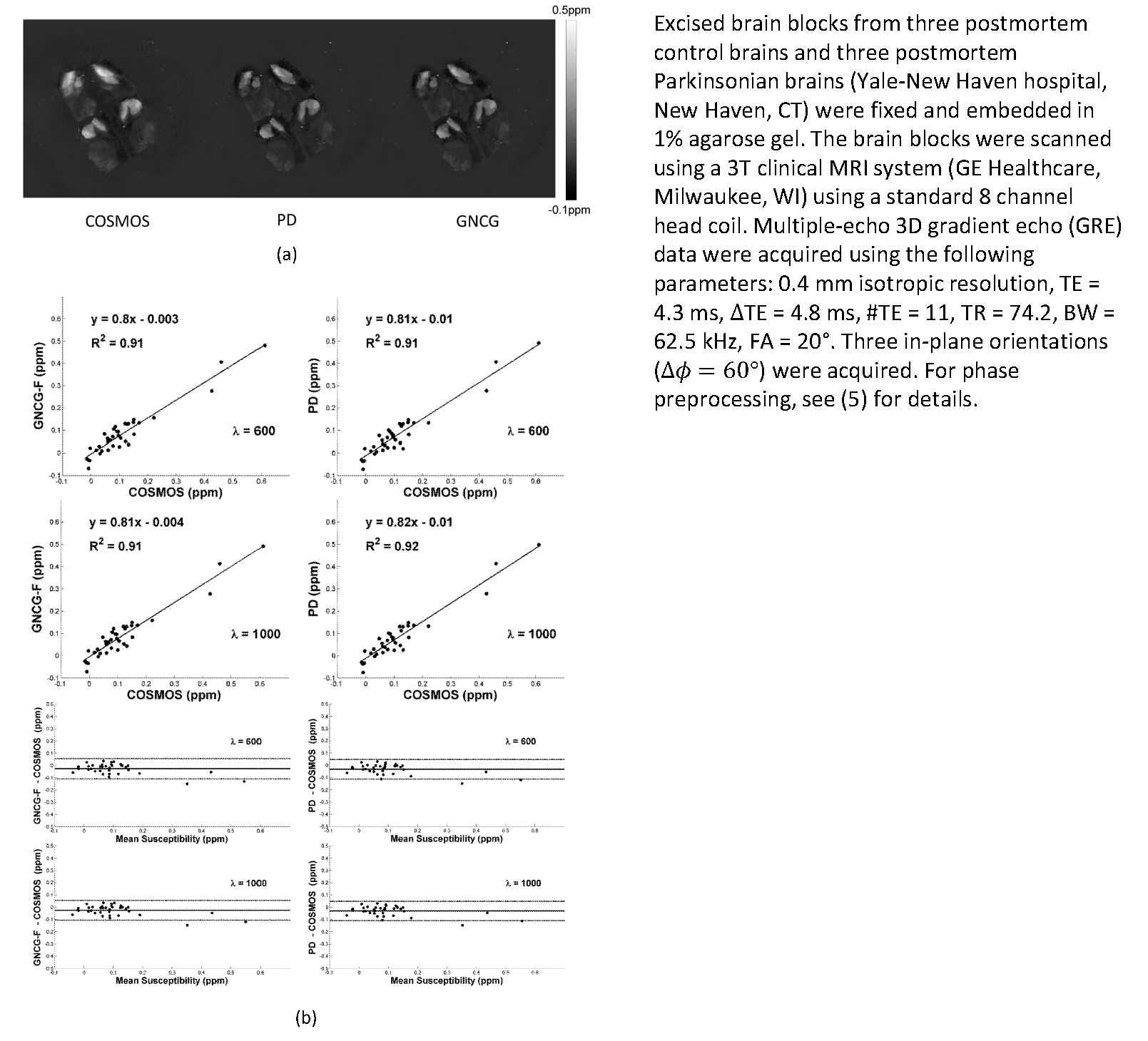
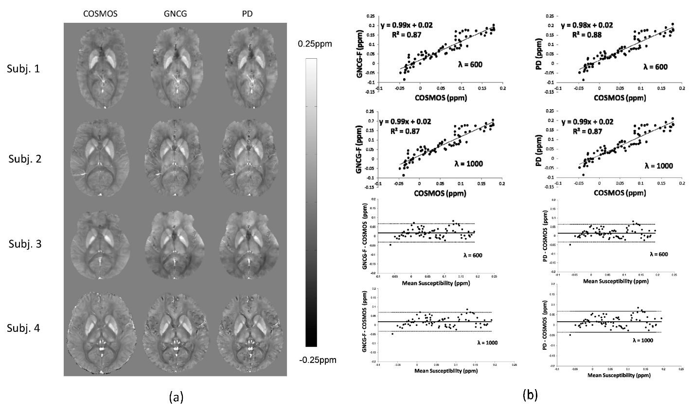
A simulated brain, in vivo brain MRI data in 4 healthy subjects, and ex vivo brain blocks were used for experimental validation of the two methods (GNCG and PD) using as reference the ground truth when available and COSMOS (4) for the healthy subjects and brain blocks. One set of the in vivo brain MRI data was downloaded at http://weill.cornell.edu/mri/pages/qsm.html. The rest of the in vivo data were extracted from (5). For phase preprocessing, see (5) for details. For the excised brain blocks, see the caption of Fig. 2 for details.

Results

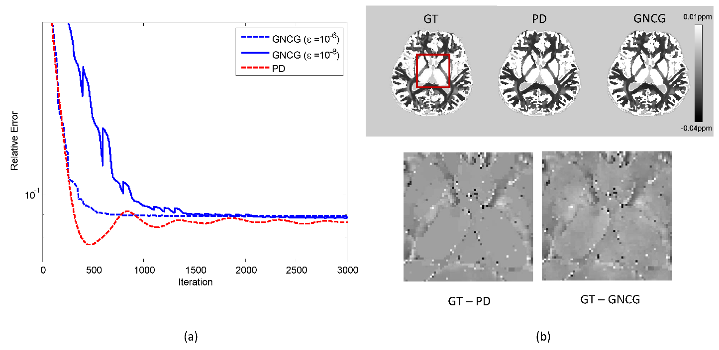
Convergence behavior of the two methods on a simulated brain is seen in Fig. 1.

Figs. 2 and 3 show the solutions obtained by the GNCG and PD algorithms and results of quantitative analysis for ex vivo brain tissues and in vivo brain data, respectively.

Discussion

The accuracy of a minimizing sequence in GNCG can be improved by decreasing $$$\epsilon$$$ from $$$10^{-6}$$$ to $$$10^{-8}$$$, but at the cost of significantly slowing down the convergence rate of the algorithm. This is because a linear system solved by the nested CG loop becomes ill-conditioned. The rate of convergence of the CG iteration is determined by the location of the eigenvalues (spectrum) of a linear system (6), and the value of the conditioning parameter $$$\epsilon$$$ affects the location of the spectrum. From a computational perspective, therefore, the algorithm would become impractical if $$$\epsilon$$$ is set to a very small number $$$\sim 10^{-10}$$$ to achieve better accuracy. This makes GNCG less preferable than PD when it comes to non-smooth convex optimization.

Conclusion

Acknowledgements

References

(1) Liu J, Liu T, de Rochefort L, Ledoux J, Khalidov I, Chen W, Tsiouris AJ, Wisnieff C, Spincemaille P, Prince MR, Wang Y. Morphology enabled dipole inversion for quantitative susceptibility mapping using structural consistency between the magnitude image and the susceptibility map. Neuroimage 2012;59(3):2560-2568.

(2) Bauschke HH, Combettes PL. Convex analysis and monotone operator theory in Hilbert spaces. CMS books in mathematics,. p 1 online resource.

(3) Chambolle A, Pock T. A first-order primal-dual algorithm for convex problems with applications to imaging. Journal of Mathematical Imaging and Vision 2011;40(1):120-145.3. Wang Y, Liu T. Quantitative susceptibility mapping (QSM): Decoding MRI data for a tissue magnetic biomarker. Magn Reson Med 2015;73(1):82-101.

(4) Wang Y, Liu T. Quantitative susceptibility mapping (QSM): Decoding MRI data for a tissue magnetic biomarker. Magn Reson Med 2015;73(1):82-101.

(5) Liu T, Liu J, de Rochefort L, Spincemaille P, Khalidov I, Ledoux JR, Wang Y. Morphology enabled dipole inversion (MEDI) from a single-angle acquisition: comparison with COSMOS in human brain imaging. Magn Reson Med 2011;66(3):777-783.

(6) Trefethen LN, Bau D. Numerical linear algebra. Philadelphia: SIAM; 1997.