1955
Evaluating The Accuracy of Susceptibility Maps Calculated from Single-Echo versus Multi-Echo Gradient-Echo Acquisitions1Medical Physics and Biomedical Engineering, University College London, London, United Kingdom, 2Leonard Wolfson Experimental Neurology Centre, Institute of Neurology, University College London, London, United Kingdom
Synopsis
For Susceptibility Mapping (SM), Laplacian-based methods (LBMs) can be used on single- or multi-echo gradient echo phase data. Previous studies have shown the advantage of using multi-echo versus single-echo data for noise reduction in susceptibility-weighted images and simulated data. Here, using simulated and acquired images, we compared the performance of two SM pipelines that used multi- or single-echo phase data and LBMs. We showed that the pipeline that fits the multi-echo data over time first and then applies LBMs gives more accurate local fields and $$$\chi$$$ maps than the pipelines that apply LBMs to single-echo phase data.
Introduction
For Susceptibility Mapping (SM), Laplacian-based methods (LBMs) can be used to perform unwrapping or background field removal of single- or multi-echo gradient echo (GRE) phase data. In previous studies on SM-LBM pipelines applied to multi-echo phase data, we have shown1,2 that fitting the multi-echo GRE phase over echo times (TEs) before applying LBMs gives more accurate local field ($$$\Delta B_{loc}$$$) and magnetic susceptibility ($$$\chi$$$) estimates than applying LBMs first and averaging over TEs. Previous susceptibility weighted imaging3 (SWI) studies on healthy volunteers and SM studies using simulations4,5 have shown that using multiple TEs reduces the propagation of phase noise into the SWI and $$$\chi$$$ images compared to using single-echo acquisitions. Here, we aimed to investigate the effect of using LBMs on single-echo phase data compared to multi-echo fitting on both $$$\Delta B_{loc}$$$ and $$$\chi$$$ accuracy. We tested two LBM-SM pipelines on simulated complex data and, unlike previous SM studies4,5, images of healthy subjects.Methods
Multi-echo 3D GRE brain images of four healthy volunteers were acquired on a Philips Achieva 3T system (Best, NL) using a 32-channel head coil and 5 echoes, TE1/ΔTE=3/5.4 ms, 1-mm isotropic resolution, TR=29 ms, FoV=240x180x144 mm3, SENSE acceleration factor in the first/second phase-encoding direction=2/1.5 and 20º flip angle.
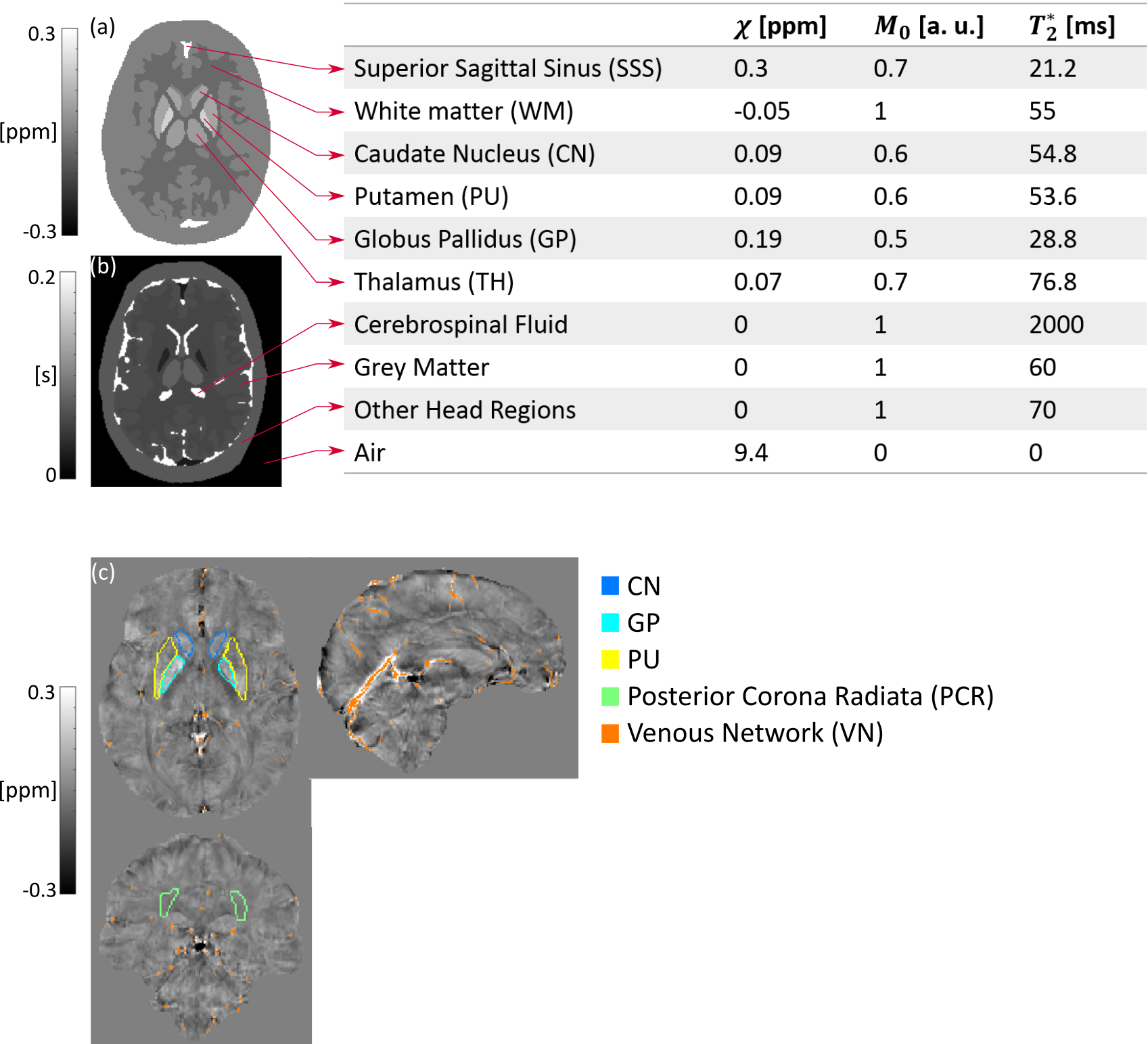
Multi-echo (5 echoes, TE1/ΔTE=3/5.4 ms) complex images were simulated from ground-truth $$$\chi^{True}$$$ (Zubal head phantom6), $$$M_0$$$ and $$$T_2^*$$$ distributions (Fig. 1), using a Fourier-based forward model7 of the total field perturbation $$$\Delta B$$$, $$$M(t)=M_0\exp(-t/T_2^*)$$$ and a constant phase offset $$$\phi_0=\pi/4$$$. Random Gaussian noise (mean = 0, standard deviation (SD) = 0.03) was added to the real and imaginary parts of the complex images to give a realistic signal-to-noise ratio. Ground-truth local field perturbation $$$\Delta B_{loc}^{True}$$$ was calculated using the reference scan method8.
$$$\Delta B_{loc}$$$ was calculated using two distinct pipelines on the phantom and volunteers’ images: 1) Multi-echo (ME): non-linear fit9 of the complex signal over TEs; $$$\Delta B_{loc}^{ME}$$$ calculation using SHARP10 ($$$\sigma=0.05$$$, BET11,12 brain mask with 2- (phantom) or 4- (volunteer) voxel erosions); 2) Single-echo (SE): at each $$$TE_i$$$, $$$\Delta B_{loc}^{SE_{i}}$$$ calculation using SHARP10 ($$$\sigma=0.05$$$, BET11,12 brain mask calculated from the i-th echo and eroded as in ME) on $$$\phi(TE_i)$$$, and dividing by $$$TE_i$$$ and $$$\gamma$$$, the gyromagnetic ratio. $$$\chi^{ME}$$$ and $$$\chi^{SE_{i}}$$$ (for i = 1 to 5) were calculated using TKD13 ($$$\delta=2/3$$$ and correction for $$$\chi$$$ underestimation10).
In the phantom, the accuracy of $$$\chi$$$ was assessed by calculating means and SDs in the regions in Fig. 1 and Root Mean Squared Errors (RMSEs) in the brain relative to $$$\chi^{True}$$$. In the volunteers, $$$\chi$$$ means and SDs were calculated in the regions in Fig. 1. All regions except VN were segmented based on the Eve $$$\chi$$$ atlas14, which was aligned to the fifth-echo magnitude image (TE5/TEEve=24.6/24 ms) using a combination of rigid, affine and non-affine transformations15,16. VN was segmented using the Multiscale Vessel Filtering method17 (scales=4, probability threshold for vein segmentation = 0.5).
Results and Discussion
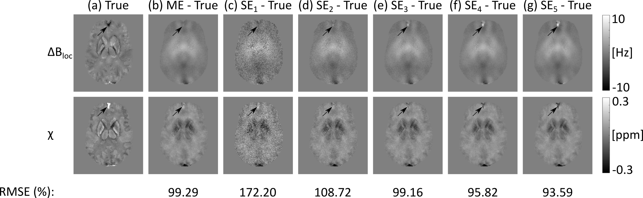
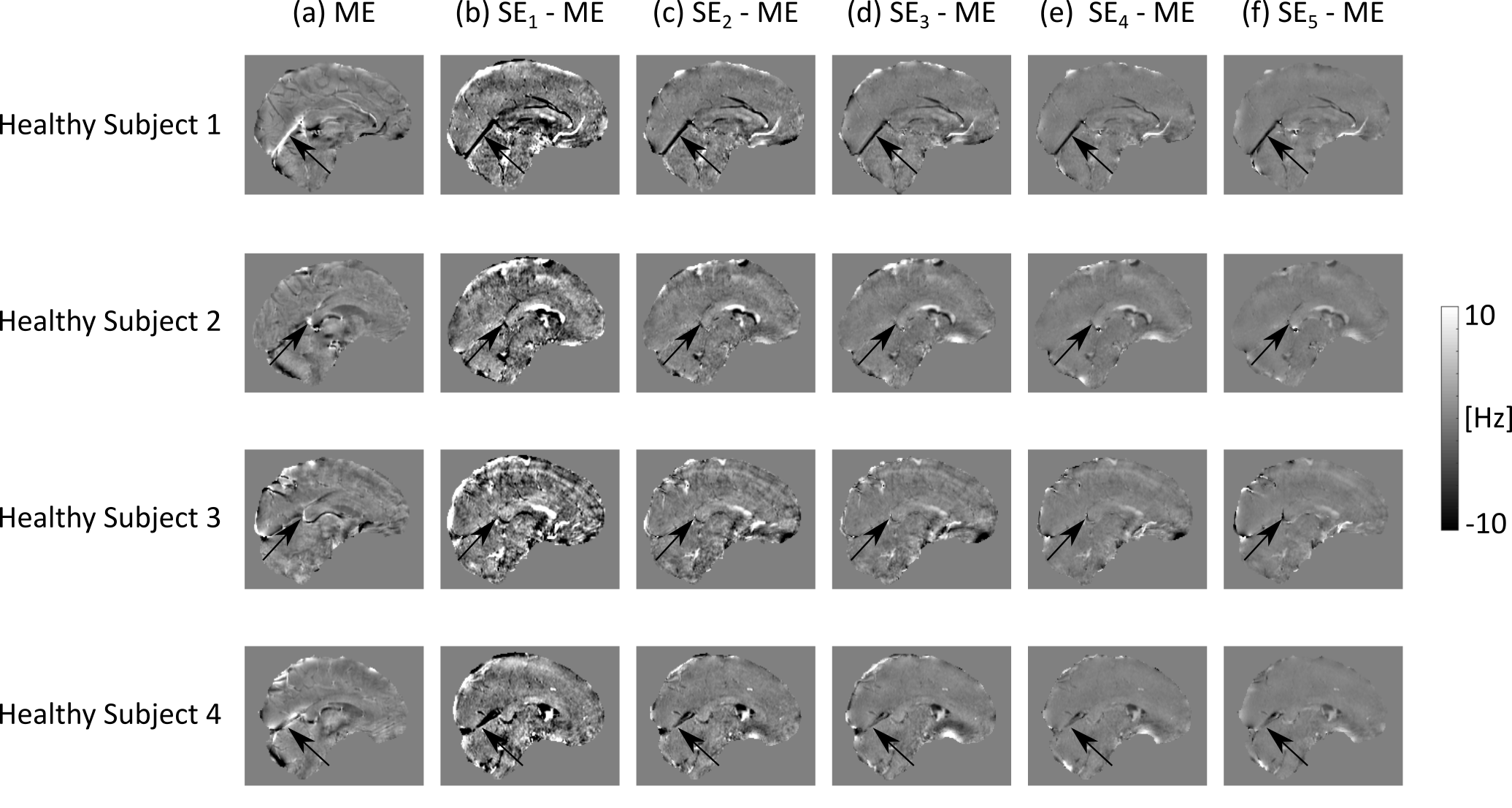
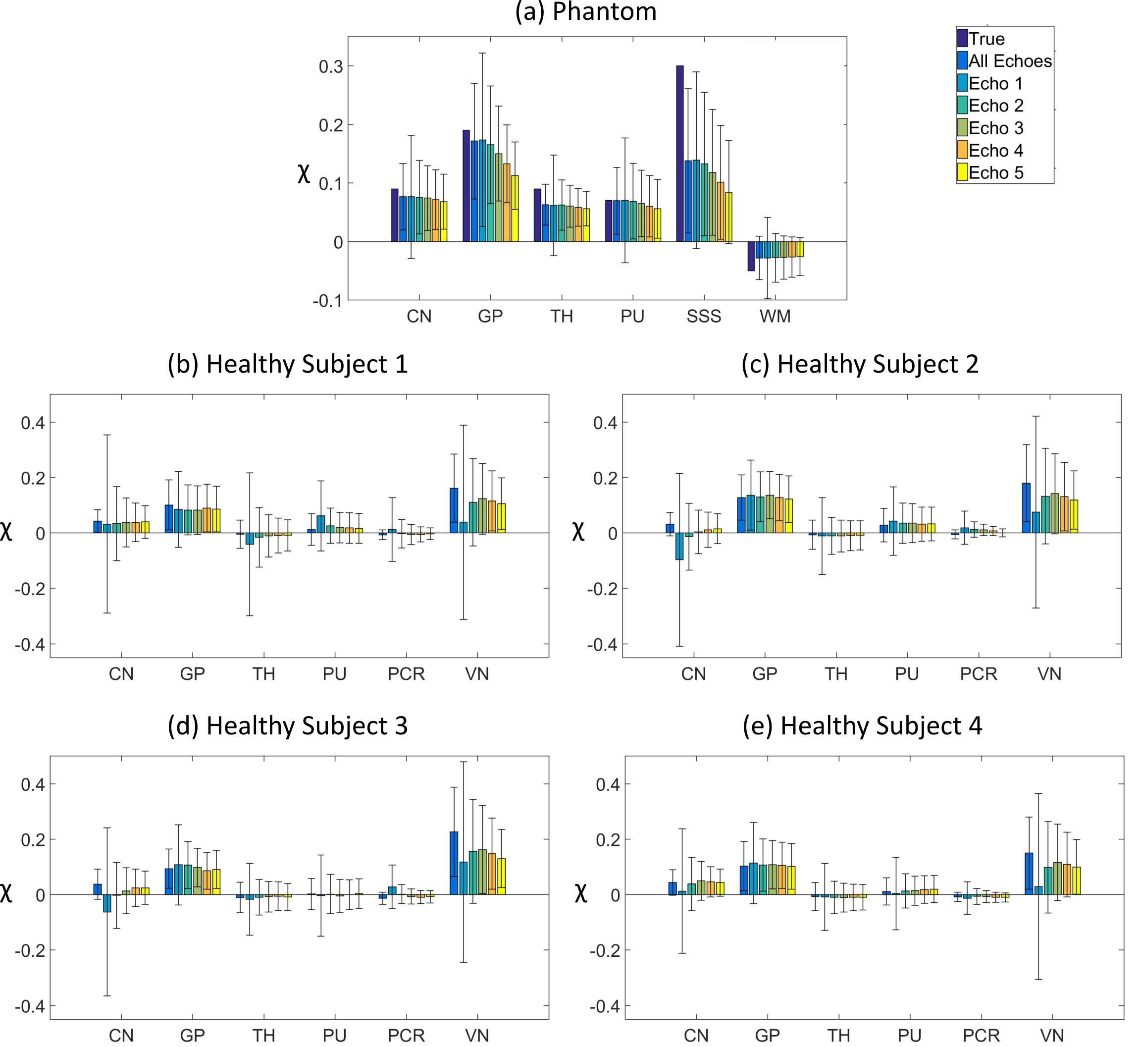
The effect of noise on the SE images decreased with increasing TE (Figs. 2c-g, 3b-f , 4b-f and SDs in Fig. 5), in line with the known relationship of the phase contrast-to-noise ratio with time: contrast-to-noise is maximised at $$$TE=T_2^*$$$ 4,5. In the phantom, mean $$$\chi^{SE_{1,2}}$$$ were similar to mean $$$\chi^{ME}$$$, but suffered from the greater noise at short TEs and had larger RMSEs than $$$\chi^{ME}$$$ (Fig. 2).
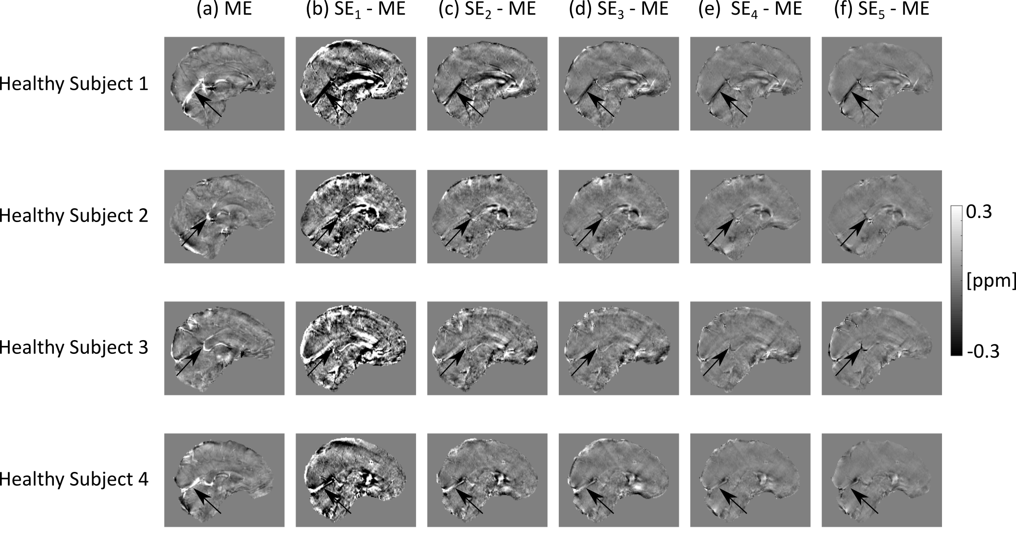
In the phantom, ME gave the most accurate $$$\Delta B_{loc}$$$ and $$$\chi$$$ estimates (Figs. 2 and 5a). High-$$$\chi$$$ structures, e.g. the SSS, showed the largest susceptibility errors in SE images, and were visible in the difference images, even at longer TEs (Figs. 2c-g). Susceptibility errors were also most prominent in the volunteers’ VN (Figs. 3b-f and 4b-f).
In the volunteers, $$$\chi^{ME}$$$ and $$$\chi^{SE_{2,3,4,5}}$$$ were approximately the same in the GP and PU (Fig. 5). However, in the other regions, only $$$\chi^{ME}$$$ always gave average values consistent with the literature13. In particular, $$$\chi^{ME}$$$ was always negative in the PCR, which is expected to be about 0.02 ppm more diamagnetic than water13,18. Furthermore, in the VN, $$$\chi^{ME}$$$ was always the closest to $$$\chi=0.46$$$ ppm, which is the expected value of $$$\chi$$$ in veins (at 70% oxygenation)19.
Conclusions
Fitting the multi-echo phase over TEs before applying LBMs gives more accurate $$$\Delta B_{loc}$$$ and $$$\chi$$$ maps than applying LBMs to single-echo phase images, particularly for high-$$$\chi$$$ structures.Acknowledgements
The authors would like to thank Dr Catarina Veiga for her help with image coregistration.References
1. Biondetti E, Thomas DL and Shmueli K. Application of Laplacian-based Methods to Multi-echo Phase Data for Accurate Susceptibility Mapping. Proc Intl Soc Mag Reson Med. 24 (2016):1547.
2. Biondetti E, Karsa A, Thomas DL et al. The Effect of Averaging the Laplacian-Processed Phase over Echo Times on the Accuracy of Local Field and Susceptibility Maps. 4th International Workshop on MRI Phase Contrast and Quantitative Susceptibility Mapping (2016)
3. Gilbert G, Savard G, Bard C et al. Quantitative comparison between a multiecho sequence and a single-echo sequence for susceptibility-weighted phase imaging. Magn Reson Imaging. 2012;30(5):722–730.
4. Wu B, Li W, Avram AV et al. Fast and tissue-optimized mapping of magnetic susceptibility and T2* with multi-echo and multi-shot spirals. NeuroImage. 2012;59(1):297–305.
5. Haacke EM, Liu S, Buch S et al. Quantitative susceptibility mapping: Current status and future directions. Magn Reson Imaging. 2015;33(1):1–25.
6. Zubal IG, Harrell CR, Smith EO et al. Two dedicated software, voxel-based, anthropomorphic (torso and head) phantoms. Proceedings of the International Conference at the National Radiological Protection Board. 1995:105–111.
7. Marques JP and Bowtell R. Application of a fourier-based method for rapid calculation of field inhomogeneity due to spatial variation of magnetic susceptibility. Concepts in Magnetic Resonance Part B: Magnetic Resonance Engineering. 2005;25(1):65–78.
8. Liu T, Khalidov I, de Rochefort L et al. A novel background field removal method for MRI using projection onto dipole fields (PDF). NMR Biomed. 2011;24(9):1129–1136.
9. Liu T, Wisnieff C, Lou M et al. Nonlinear formulation of the magnetic field to source relationship for robust quantitative susceptibility mapping. Magn Reson Med. 2013;69(2):467–476.
10. Schweser F, Deistung A, Sommer K et al. Toward online reconstruction of quantitative susceptibility maps: Superfast dipole inversion. Magnetic Resonance in Medicine. 2013;69(6):1582–1594.
11. Jenkinson M, Beckmann CF, Behrens TEJ et al. Fsl. NeuroImage. 2012;62(2):782–790.
12. Smith SM. Fast robust automated brain extraction. Hum Brain Mapp. 2002;17(3):143–155.
13. Shmueli K, de Zwart JA, van Gelderen P et al. Magnetic susceptibility mapping of brain tissue in vivo using MRI phase data. Magn Reson Med. 2009;62(6):1510–1522.
14. Lim IAL, Faria A V., Li X et al. Human brain atlas for automated region of interest selection in quantitative susceptibility mapping: Application to determine iron content in deep gray matter structures. NeuroImage. 2013;82:449–469.
15. Ourselin S, Roche A, Subsol G et al. Reconstructing a 3D structure from serial histological sections. Image Vis Comput. 2001;19(1–2):25–31.
16. Modat M, Ridgway GR, Taylor ZA et al. Fast free-form deformation using graphics processing units. Comput Methods Programs Biomed. 2010;98(3):278–284.
17. Bazin PL, Plessis V, Fan AP et al. Vessel segmentation from quantitative susceptibility maps for local oxygenation venography. ISBI 2016:1135–1138.
18. Duyn JH, Schenck J. Contributions to magnetic susceptibility of brain tissue. NMR in Biomed. 2016.
19. Fan AP, Bilgic B, Gagnon L et al. Quantitative oxygenation venography from MRI phase. Magn Reson Med. 2014;72(1):149–159.
Figures