1954
Susceptibility Mapping Reveals Inter-Hemispheric Differences in Venous Density in Patients with Brain Arteriovenous Malformations1Medical Physics and Biomedical Engineering, University College London, London, United Kingdom, 2Brain Repair and Rehabilitation, Institute of Neurology, University College London, London, United Kingdom, 3Leonard Wolfson Experimental Neurology Centre, Institute of Neurology, University College London, London, United Kingdom
Synopsis
Brain arteriovenous malformations (AVMs) are vascular abnormalities characterised by arteriovenous shunting with the lack of a capillary bed. Recent studies have shown that it is possible to create diagrams of the cerebral vein network (venograms) from images of magnetic susceptibility ($$$\chi$$$). Here, we used $$$\chi$$$-based venograms to calculate the hemispheric percentage of venous voxels (venous density) in each hemisphere in AVM patients and healthy subjects. We found larger venous densities in the AVM-containing hemispheres than in the contralateral hemispheres, and more variable venous density in AVM patients than in healthy subjects.
Introduction
Brain arteriovenous malformations (AVMs) are characterised by anomalous connections between arteries and veins leading to arteriovenous shunting through a network of coiled and tortuous vessels, the so called nidus, without a normal intervening capillary bed. This arteriovenous shunt causes abnormal blood flow in and around AVMs and the presence of more oxygenated, higher pressure blood in the draining veins1,2.
Recent studies3-7 have exploited the bright appearance of paramagnetic deoxygenated venous blood in maps of magnetic susceptibility ($$$\chi$$$) to create diagrams of the cerebral vein network (venograms).
Here, we present the first results of a study on AVM pathophysiology in a cohort of patients, each with an untreated brain AVM. We investigated the vascularisation in the two cerebral hemispheres by calculating hemispheric venous density (VD) from $$$\chi$$$-based venograms.
Methods
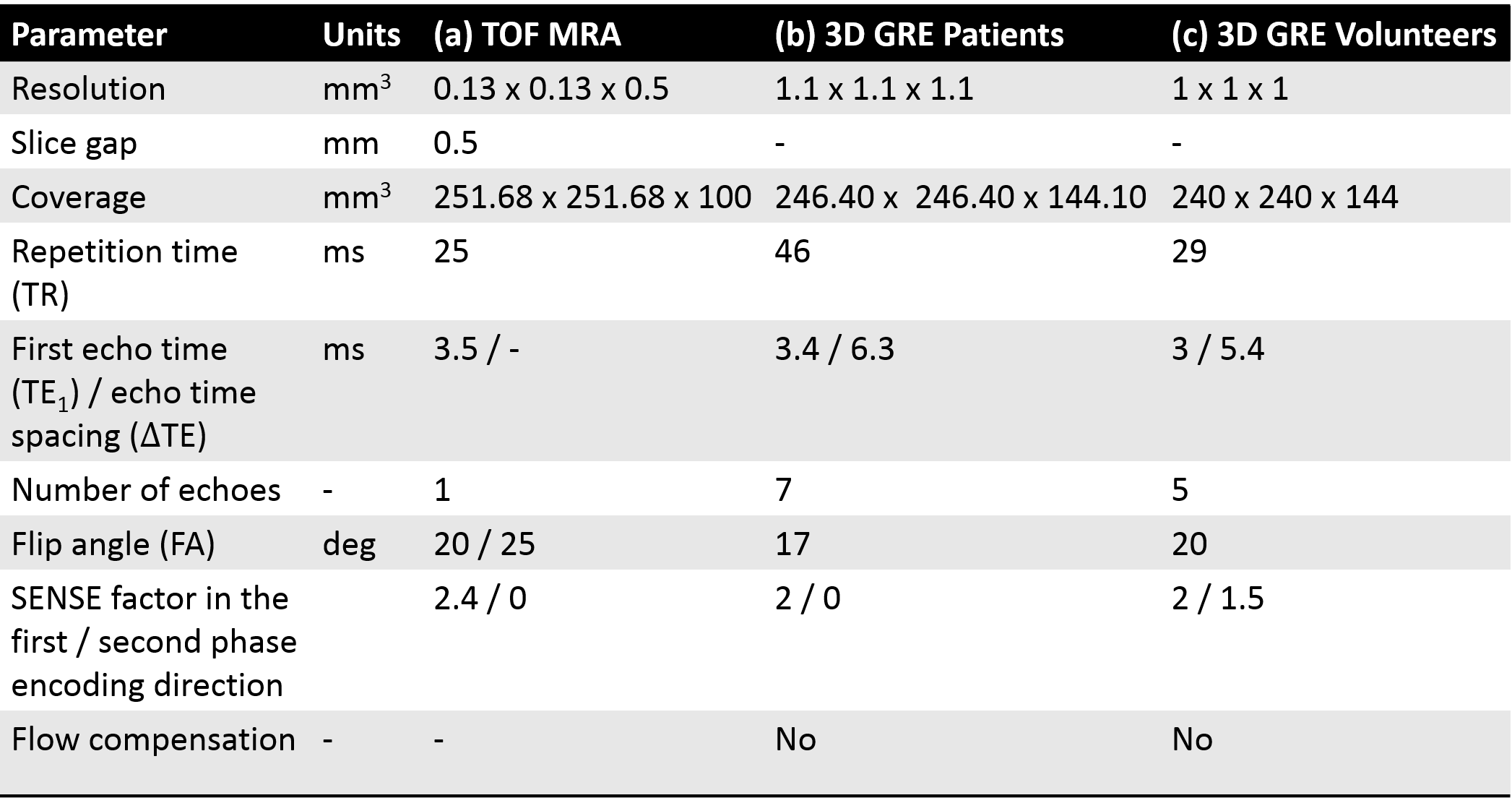
Fourteen patients (age: 38±14 years) and four healthy volunteers (HVs) were scanned with a Philips Achieva 3T system (Best, NL) using a 32-channel head coil. Patients were scanned using an axial time-of-flight (TOF) magnetic resonance angiography (MRA) acquisition (Table 1a) and a whole-brain 3D multi-echo (ME) gradient-echo (GRE) sequence for susceptibility mapping (SM) (Table 1b). The volunteers were scanned using a slightly different 3D ME GRE sequence for SM (Table 1c).
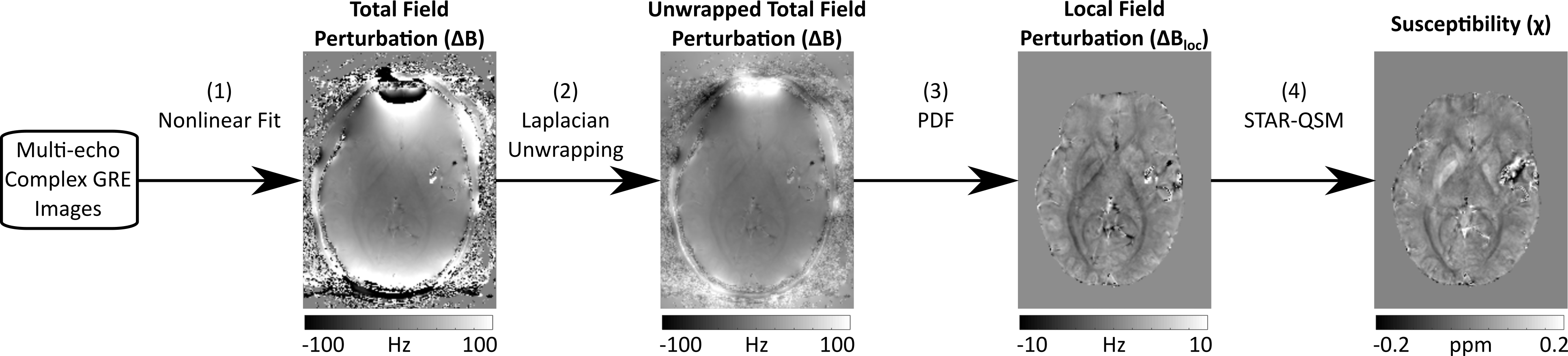
For each subject, the $$$\chi$$$ map was calculated as described in Fig. 1. The left (LH) and right hemispheres (RH) were segmented based on the Eve atlas15, which was aligned to each patient’s fourth and each volunteer’s fifth GRE magnitude image (TE4,patients/TE5,volunteers/TEEve = 22.3/24.6/24 ms) using a combination of rigid, affine and non-affine transformations16,17.
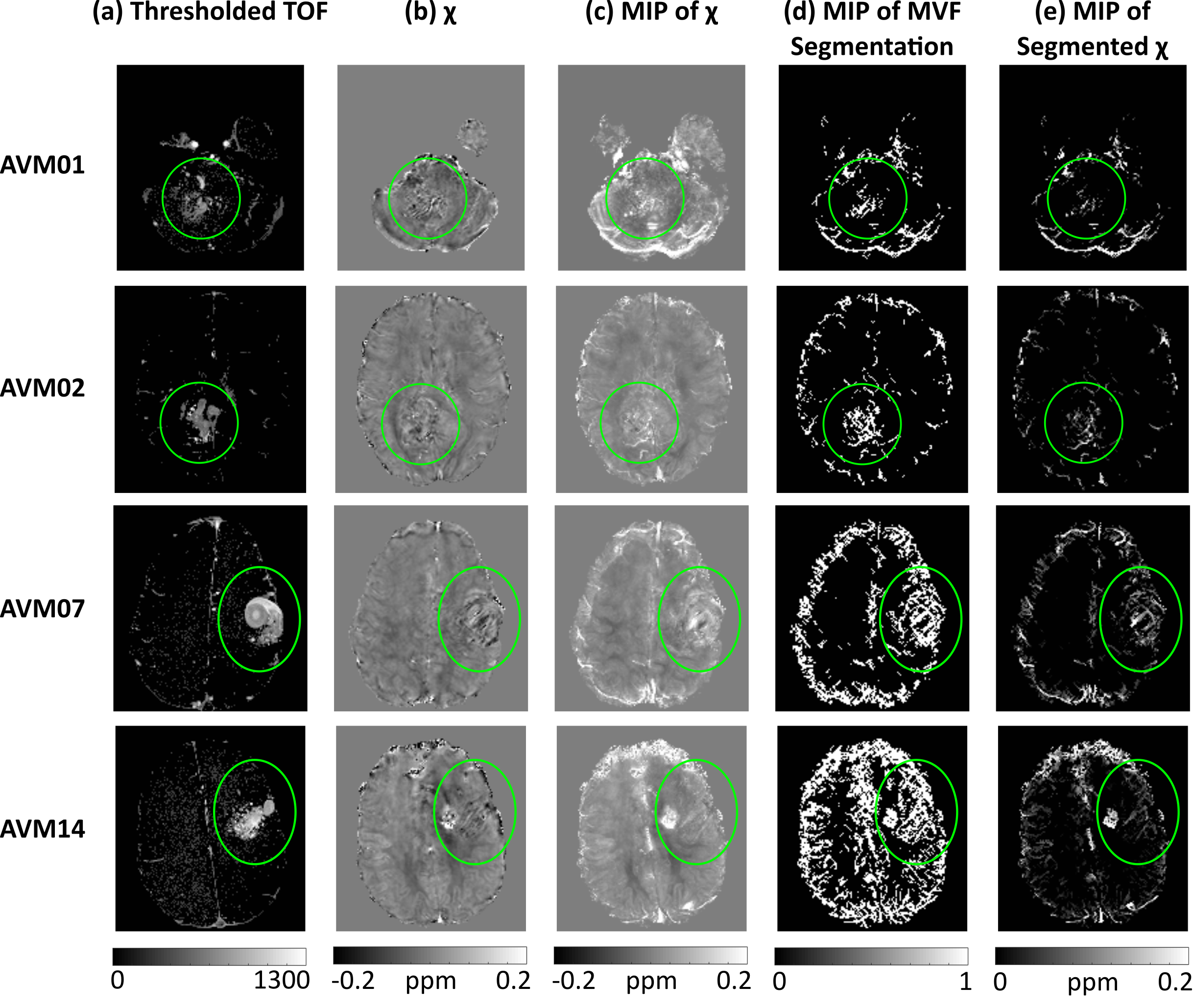
$$$\chi$$$-based venograms of patients and HVs were calculated using probabilistic Multiscale Vessel Filtering6 (MVF) (10 scales). Veins were segmented by thresholding the probability map $$$p$$$ at $$$p(vein) \geq 0.5$$$. To better appreciate the vasculature, transverse Maximum Intensity Projections (MIPs) of the $$$\chi$$$ maps, vein segmentations and segmented $$$\chi$$$ maps were calculated across slabs of ten slices.
In the patients, the TOF images were rigidly coregistered16 to the first-echo GRE magnitude image and then thresholded at a fixed intensity to highlight bright vessels. The thresholded TOF images were used to delineate the vessel network in and around the AVM, and to locate the AVM in the $$$\chi$$$ maps.
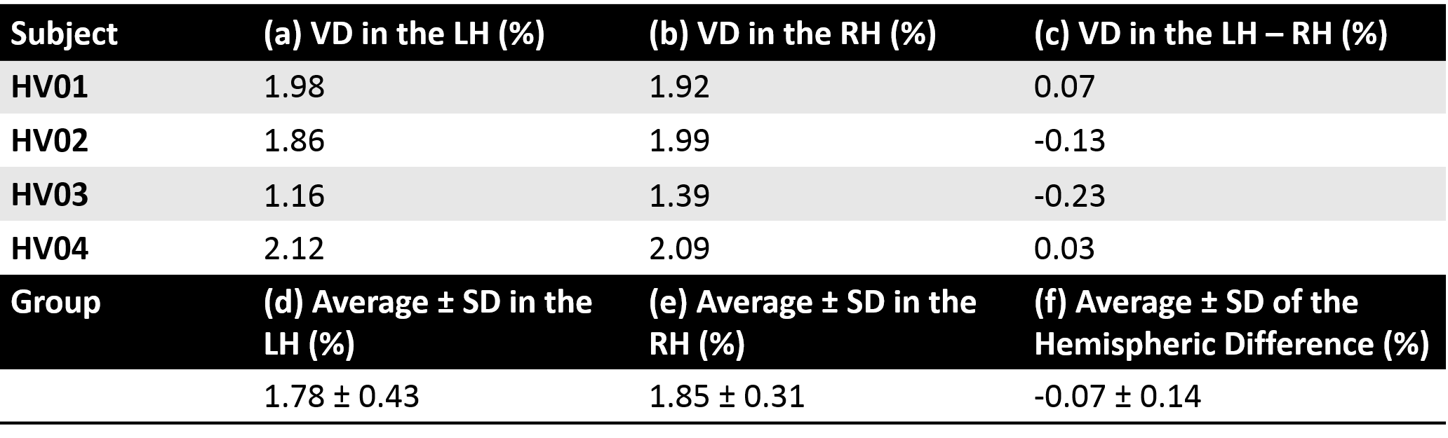
VD was calculated in each subject’s LH and RH as the ratio (%) between the number of MVF-segmented “venous” voxels and the total number of voxels in each hemisphere. The VD in both hemispheres as well as the inter-hemispheric difference was calculated in each subject, along with group-wise means and standard deviations (SDs).
Results and Discussion
Figs. 2a and b show that it is possible to locate some AVM features in both TOF images and $$$\chi$$$ maps, despite possible SM confounds due to the lack of flow compensation. Vessels highlighted in the TOF images and appearing bright in the $$$\chi$$$ maps could be AVM draining veins. However, the AVMs’ feeding arteries and the arterial side of the AVMs’ nidi are probably only visible in the TOF images. These arterial features, as well as draining veins containing mixed arterial and venous blood, are likely to be less visible in the $$$\chi$$$ map because arterial blood and the surrounding brain parenchyma are both similarly diamagnetic. Notably, the bright veins in Fig. 2c appear well delineated in Fig. 2d and e.
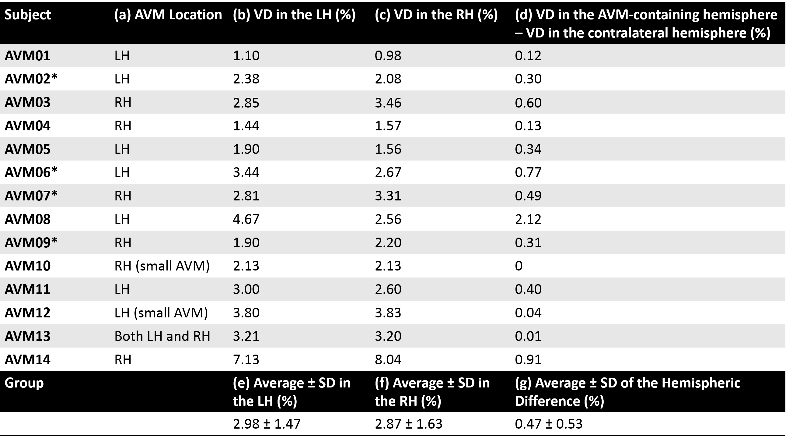
Tables 2 and 3 show the VD measurements in the patients and volunteers respectively. In the patients, the hemisphere containing the AVM (Table 2a) always had the largest VD (Table 2d) except in patients AVM10, AVM12 and AVM13, in which the AVM was small or located in both hemispheres. The average inter-hemispheric VD difference was larger in the patients (Table 2g) than in the HVs (Table 3f). Furthermore, the VD average ± SD was always larger in the patients (Table 2e-g) than in the HVs (Table 3d-f).
Although haemorrhage by-products, such as paramagnetic haemosiderin, might have contributed to increased VD by being erroneously included in the MVF segmentations, the fact that four patients (starred in Table 2) did not have a previous bleed suggests that the increased VD of the AVM-containing hemisphere is mostly driven by increased vascularisation.
Conclusions and Future Work
We have shown that $$$\chi$$$ maps can be used to calculate hemispheric VD. We report larger VD in the AVM-containing hemisphere than in the contralateral hemisphere, and an increased variability in VD in AVM patients compared to healthy subjects. This interesting information about AVM physiology might have implications for the automated detection of brain AVMs.
Future work will involve investigating the venous oxygenation ($$$SvO_2$$$) in this cohort of patients relative to $$$SvO_2$$$ in HVs.
Acknowledgements
The authors would like to thank Dr Audrey Fan and Dr Pierre-Louis Bazin for their help with vessel segmentation, and Dr Catarina Veiga for her help with image coregistration.References
1. Dillon WP. Cryptic vascular malformations: Controversies in terminology, diagnosis, pathophysiology, and treatment. Am J Neuroradiol. 1997;18(10):1839–1846.
2. Friedlander RM. Arteriovenous Malformations of the Brain. N Engl J Med. 2007;356(26):2704–2712.
3. Serres B, Deistung A, Schäfer A et al. Automatic Segmentation of the Venous Vessel Network Based on Quantitative Susceptibility Maps and its Application to Investigate Blood Oxygenation. Proc Intl Soc Mag Reson Med. 23. (2015):0169.
4. Fan AP, Bilgic B, Gagnon L et al. Quantitative oxygenation venography from MRI phase. Magn Reson Med. 2014;72(1):149–159.
5. Xu B, Liu T, Spincemaille P et al. Flow compensated quantitative susceptibility mapping for venous oxygenation imaging. Magn Reson Med. 2014;72(2):438–445.
6. Bazin PL, Plessis V, Fan AP et al. Vessel segmentation from quantitative susceptibility maps for local oxygenation venography. ISBI 2016:1135–1138.
7. Ward PGD, Raniga P, Ferris NJ et al. Venous metrics in a large cohort of healthy elderly individuals from susceptibility-weighted images and quantitative susceptibility maps. Proc Intl Soc Mag Reson Med. 24 (2016):0329.
8. Liu T, Wisnieff C, Lou M, et al. Nonlinear formulation of the magnetic field to source relationship for robust quantitative susceptibility mapping. Magn Reson Med. 2013;69(2):467–476.
9. Schweser F, Deistung A, Sommer K et al. Toward online reconstruction of quantitative susceptibility maps: Superfast dipole inversion. Magn Reson Med. 2013;69(6):1582–1594.
10. Value chosen as in the Matlab MEDI Toolbox v. 02/02/2016, function unwrapLaplacian.m.
11. Liu T, Khalidov I, de Rochefort L et al. A novel background field removal method for MRI using projection onto dipole fields (PDF). NMR Biomed. 2011;24(9):1129–1136.
12. Jenkinson M, Beckmann CF, Behrens TEJ et al. Fsl. NeuroImage. 2012;62(2):782–790.
13. Smith SM. Fast robust automated brain extraction. Hum Brain Mapp. 2002;17(3):143–155.
14. Wei H, Dibb R, Zhou Y et al. Streaking artifact reduction for quantitative susceptibility mapping of sources with large dynamic range. NMR Biomed. 2015;28(10):1294–1303.
15. Lim IAL, Faria A V., Li X et al. Human brain atlas for automated region of interest selection in quantitative susceptibility mapping: Application to determine iron content in deep gray matter structures. NeuroImage. 2013;82:449–469.
16. Ourselin S, Roche A, Subsol G et al. Reconstructing a 3D structure from serial histological sections. Image Vis Comput. 2001;19(1–2):25–31.
17. Modat M, Ridgway GR, Taylor ZA et al. Fast free-form deformation using graphics processing units. Comput Methods Programs Biomed. 2010;98(3):278–284.
Figures