Synopsis

This study explores the opportunity of using ultra-high field (21.1 T) for producing electrical conductivity maps. Phantoms with known NaCl concentrations were used to compare conductivity maps generated by phase-based MREPT with actual values measured at 900 MHz with a dielectric probe. Phase-based MREPT also was evaluated for in vivo ischemic brain using an MCAO rat model. Increased conductivity values were noted in the stroked region of the rat brain.

Introduction

Materials and Methods

Phantoms with different salt concentrations were evaluated as well as brain tissue in healthy rats and diseased rats that have experienced cerebral ischemia. The phase-based method has been used for initial conductivity calculations.

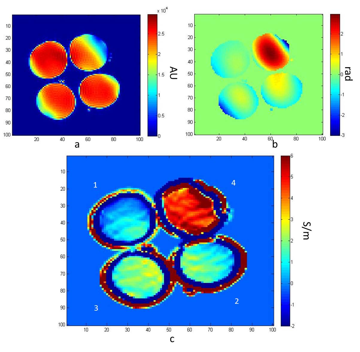
Phantom: Four 3-mL plastic transfer pipettes contained solutions doped with 1.5 g/L CuSO₄ but different NaCl concentrations: 2 g/L, 6 g/L, 12 g/L and 36 g/L. The actual conductivity values measured with an HP 85070C dielectric probe were 0.63, 1.31, 2.09 and 5.13 S/m, respectively.

Stroke model: To investigate brain ischemia, middle cerebral artery occlusion (MCAO) was performed on three 150-g Sprague-Dawley rats for 1-h followed by re-perfusion. They were imaged 24 h following MCAO.

MR Acquisitions: Data were acquired at the National High Magnetic Field Laboratory (NHMFL) using a 21.1-T vertical magnet and a linear birdcage RF coil (35.5-mm diameter) operating at 900 MHz. 2D spin echo (SE) sequences were acquired with a TE/TR of 9.5/3000 ms, resolution of 400x400x1000 µm³ and 10 slices for the phantom study. In vivo measurements used fast spin-echo (FSE) acquisitions with TE/TR of 13/6000 ms, resolution of 100x100x500 mm³ and 25 slices. Axial images were acquired with two averages and a RARE factor of four. Total scan time was 15 min.

Data Processing: Starting with the homogenous Helmholtz equation for a region with constant conductivity and estimating phase transmit φ⁺ as half of the transceive phase (φ_t), conductivity was calculated using:

$$\sigma=\frac{1}{\mu_0\omega}\nabla^2\phi_t(r),$$

where µ₀ is free space magnetic permeability and ω is the angular frequency (rad/s). To take the 3D Laplacian in MATLAB, the 3D image phase was convolved with three noise-robust kernels for each direction. The summation of these three directions yielded the 3D Laplacian. Due to tissue heterogeneity and boundaries, a 5x5 median filter was used for smoothing the in vivo conductivity maps to provide cleaner representations.

Results and Discussion

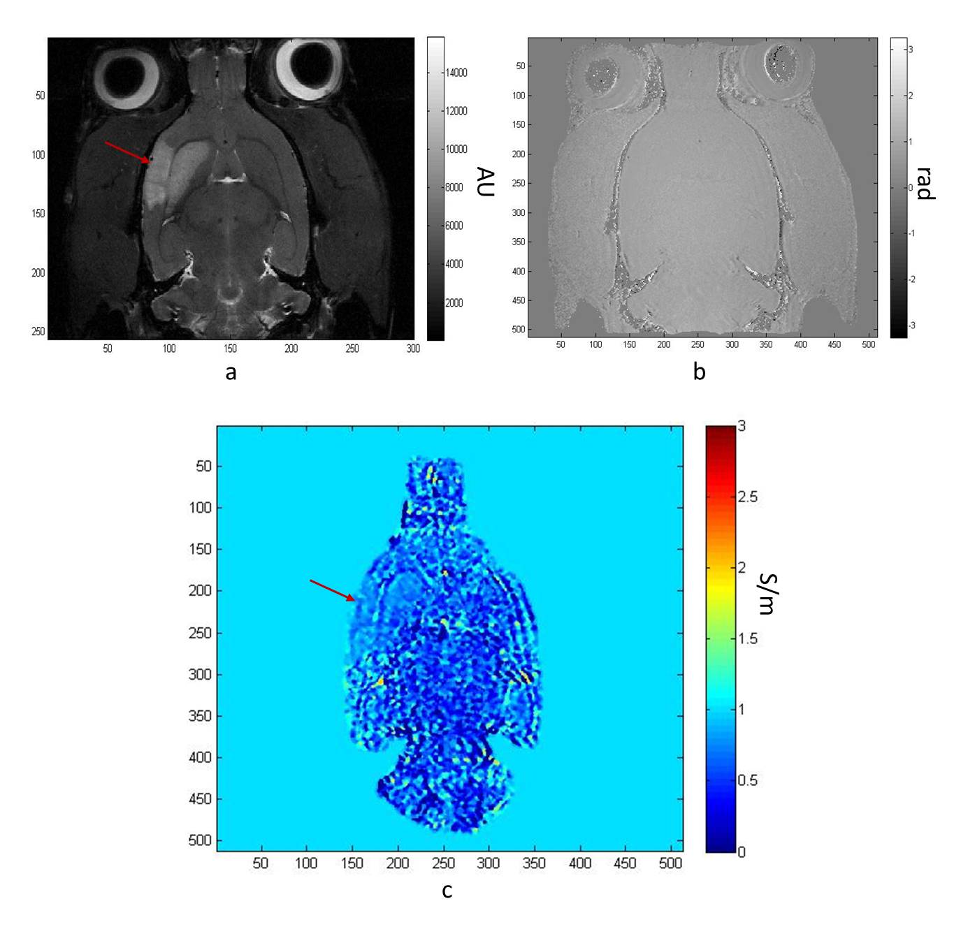
Figures 1 shows SE magnitude, phase and conductivity maps of the phantom, respectively. Figures 2 shows the FSE magneitude, phase and conductivity maps for an MCAO rat, respectively, with the stroke indicated by the red arrow. Average conductivity values were determined for the solutions: σ₁=0.49 ± 0.59 S/m; σ₂=1.38 ± 0.55 S/m; σ₃=1.92 ± 0.41 S/m; σ₄=4.93 ± 0.68 S/m, which showed agreement with expected values but larger variation for low conductivities. Conductivity values in the MCAO brain (Figure 4) were: stroke region σ=0.75 ± 0.14 S/m and contralateral side σ=0.6± 0.27 S/m).

Based on these phantom experiments, it was determined that a 3x7x5 matrix for the noise-robust kernel used to process the discrete Laplacian was suitable, in agreement with previous reports³. This kernel also was employed for in vivo images.

In phantoms images at 21.1 T, the B₁⁺ phase assumption tends to underestimate expected conductivity values, but these values seem to deviate from the expected conductivity less than previous studies conducted at 7 T⁴.

For in vivo images, the average conductivity in the stroked region was notably 25% higher than the contralateral side. Boundary artifacts resulting from the combination of the Helmholtz equation and discrete calculation of Laplacian were visible around the tubes and particularly between tissue boundaries in the brain.

Conclusions and Future Work

Electrical conductivity mapping using only B₁⁺ phase is possible in piecewise constant dielectric regions, because the reconstruction is directly based on application of the homogenous Helmholtz equation in uniform regions. Dielectric properties and inhomogeneous RF field propagation are responsible for inhomogeneous phase distribution at higher fields. However, it was observed that using a small RF coil relative to the RF wavelength (λ=36 mm in pure water at 900 MHz) helped to reduce RF inhomogeneities that could negatively impact conductivity maps.

In ongoing studies, the influence of neglecting B₁⁺ amplitude in the Helmholtz equation is being evaluated, and different techniques to reduce boundary artifacts and increase noise robustness will be investigated. This study can be used as a step toward more accurate in vivo conductivity mapping at high fields, particularly under pathological conditions.

Acknowledgements

References

1. E. M. Haacke, L. S. Petropoulos, E. W. Nilges, D. H. Wu. 1991. Extraction of conductivity and permittivity using magnetic resonance imaging. Phys. Med. Biol. 36(6): 723–734.

2. U. Katscher, T. Voigt, C. Findeklee, P. Vernickel, K. Nehrke, O. Dössel. 2009. Determination of electric conductivity and local SAR via B1 mapping. IEEE Trans. Med. Imaging. 28(9): 1365–1374.

3. A. L. H. M. W. Van Lier, D. O. Brunner, K. P. Pruessmann, D. W. J. Klomp, P. R. Luijten, J. J. W. Lagendijk, C. A. T. Van Den Berg. 2012. B1+ phase mapping at 7 T and its application for in vivo electrical conductivity mapping. Magn. Reson. Med. 67(2): 552–561.

4. A. L. H. M. W. Van Lier, A. Raaijmakers, T. Voigt T, J.J. Lagendijk JJ, P.R. Luijten, U. Katscher, C.A.T. Van Den Berg. 2014. Electrical properties tomography in the human brain at 1.5, 3, and 7T: a comparison study. Magn. Reson. Med. 71(1): 354–363.