1949
Use of Padding to Eliminate Low Convective Field Artifact in Conductivity Maps Obtained by cr-MREPT1Electrical and Electronics Engineering, Bilkent University, Ankara, Turkey
Synopsis
Convection-reaction equation based Magnetic Resonance Electrical Properties Tomography (cr-MREPT) has been developed by Hafalir et.al; however Low Convective Field causes artifacts. This study investigates how padding can be used in practice to eliminate the LCF artifact in conductivity reconstructions. Simulation and experimental results are given to demonstrate that conductivity images are improved by padding.
Introduction
Convection-reaction equation based Magnetic Resonance Electrical Properties Tomography (cr-MREPT) has been developed by Hafalir et.al. and use of pads for removal of Low Convective Field (LCF) artifacts has been proposed1. This study investigates how padding can be used in practice to eliminate the LCF artifact in conductivity reconstructions. Simulation and experimental results are given to demonstrate that conductivity images are improved by padding.Methods
Simulations are conducted in a birdcage body coil model using Comsol Multiphysics (COMSOL AB, Stockholm, Sweden). Figure 1 shows the simulation phantom containing four different regions: B and C represent anomaly regions with conductivity of 1S/m and 1.5S/m respectively, placed in the background region A with conductivity of 0.5S/m. The relative dielectric constants ($$$\epsilon_{r}$$$) of A, B and C are taken as 80. D is the padding material for which $$$\epsilon_{r}$$$ is taken as 1 (no pad condition), 80 and 350 in 3 different simulations.
For MRI experiments, Siemens Tim Trio 3T MR scanner (Erlangen, Germany) with a quadrature body coil (transmit and receive) is used. A rectangular pad (24cmx18cmx1cm) containing water ($$$\epsilon_{r}$$$= 80) is prepared and wrapped around the cylindrical phantom during the experiments. 3 different experiments are conducted consecutively: without pad, pad positioned on the left-side and on the right-side. 2D-SSFP (FoV=150mm, 1.2mmx1.2mmx3.0mm, FA=40°, TE/TR=2.44ms/4.88ms,duration=6.4min) is used to obtain B1 phase, and GRE (FoV=150mm, 1.2mmx1.2mmx3.0mm, FA=60°/120°, TE/TR=5ms/5000ms, duration=10.2min) is used for B1-mapping via the Double-Angle method. Noise is reduced using PDE-based diffusion filtering.
The cr-MREPT PDE is as follows: $$$\it F\cdot\overline{\triangledown}u+\triangledown^{2}H^{+}u-i\omega\mu_{0}H^{+}=0$$$, where $$$u=\frac{1}{\sigma+iw\epsilon_{0}\epsilon_{r}}$$$ is the unknown admittance, $$$H^{+}$$$ is transmit magnetic field from the simulation and experiment results. Since our phantoms are z-independent, partial derivatives w.r.t. z are zero; thus the calculation of the coefficients of the PDE and solution of cr-equation itself is done for 2D on a triangular mesh for the slice of interest2. In the 2D formulation $$$F=\begin{bmatrix}F_{x} \\F_{y} \end{bmatrix} = \begin{bmatrix} \frac{\partial H^{+}}{\partial x}-i\frac{\partial H^{+}}{\partial y} \\i\frac{\partial H^{+}}{\partial x}+\frac{\partial H^{+}}{\partial y} \end{bmatrix}$$$ is the convective field, where $$$F_{x}=iF_{y}$$$. The cr-MREPT equation is converted to a linear algebraic system of equations. Conductivity reconstructions have artifacts at the regions where convective field is very low. Dielectric pad shifts the LCF region (low $$$F$$$ region), providing us data sets with different LCF regions. These different data sets are solved simultaneously and the method eliminates the LCF artifact in the ROI if the convective field is high in that region in at least one of the data sets.
Results
Conductivity reconstructions for the simulation phantom for the no-pad, left and right $$$\epsilon_{r}$$$= 80 pads are shown in Figure 2. The corresponding LCF regions are also shown, with the magnitude of Fx is plotted such that its values are thresholded at a low value to emphasize the positions of the LCFs. With opposite pad locations, LCF region and the LCF artifact shift in opposite directions. Figure 3 shows the conductivity maps and LCF regions for $$$\epsilon_{r}$$$= 350 pad case. Amount of the shifts (in mm) in LCF regions are given in the figure captions. In general, $$$\epsilon_{r}$$$= 350 pads shift LCF more than the $$$\epsilon_{r}$$$= 80 pads. Conductivity maps obtained by combining different data sets are given in Figure 4. Combining the $$$\epsilon_{r}$$$= 350 left and right pads' data gives the best result; eliminating the LCF artifact and yielding correct conductivity values.
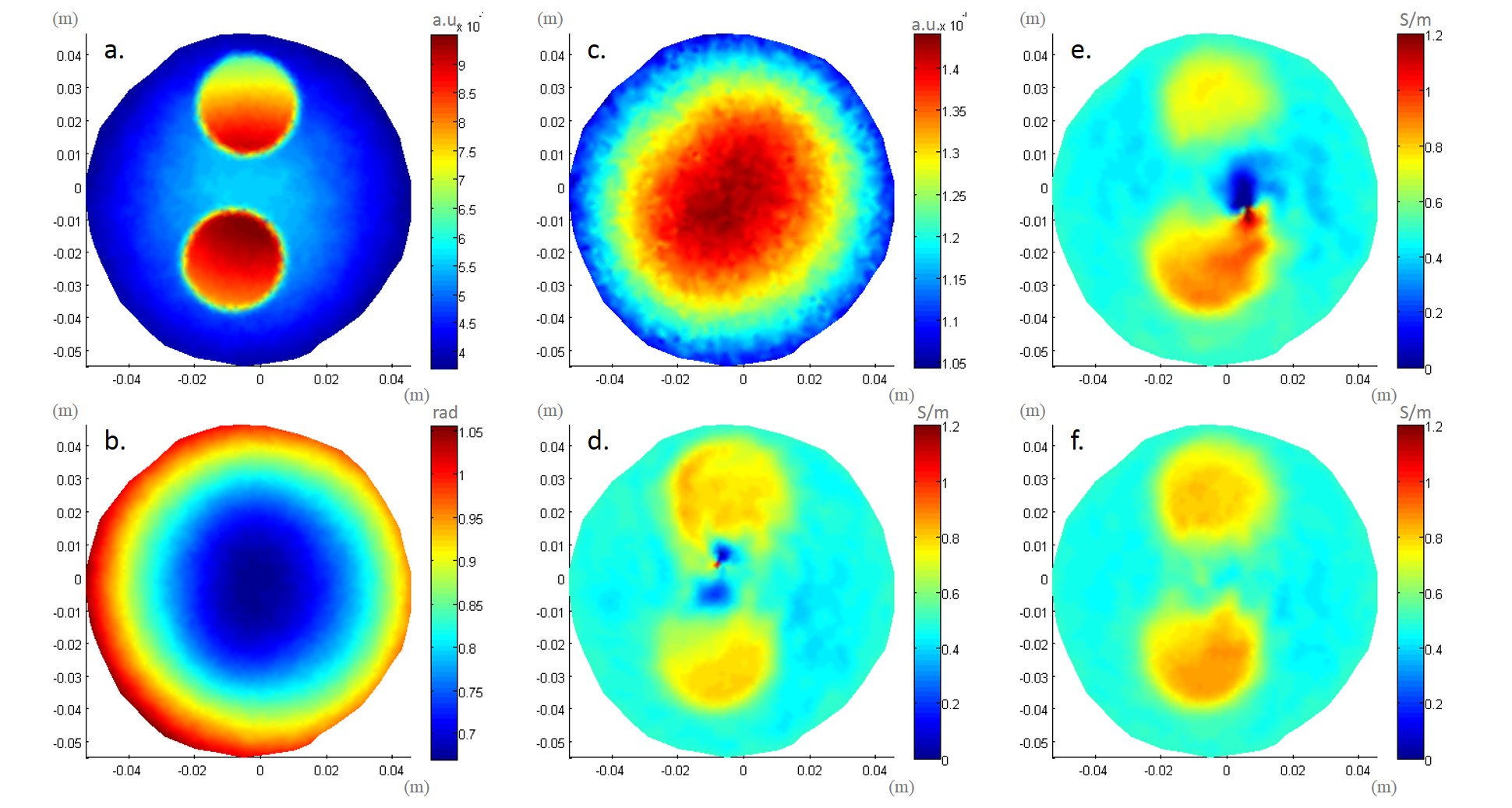
SSFP magnitude and phase images, and the B1-map as well as the conductivity reconstructions obtained from the experimental phantom are given in Figure 5. Amount of shifts in experiments are similar to simulations. However, experimental noise widens the LCF regions and therefore the two LCFs (from left-sided and right-sided pads) overlap. Combining the data from these two cases eliminates the LCF artifact but the reconstruction is distorted due to noise.
Discussion and Conclusion
Our experimental results are inline with the simulation results. However, to reduce the effect of the measurement noise, especially the B1 magnitude had to be heavily filtered. This filtering smooths the images but more error is induced in the conductivity values. Our future studies will cover experiments with high dielectric pads such as Barium Titanate3 slurries in order to increase the LCF shifts, and thereby making the method more robust against noise.
Simulations and experiments with different pad structures have also been conducted. In general, positioning the pad closer to phantom shifts the LCF region more. Thinner and thicker pads compared to current ones shift the LCF region less. Very high dielectric values disturbs the field undesirably. Small pads, which do not cover at least half the phantom surface do not shift LCF sufficiently.
Acknowledgements
This study was supported by TUBITAK 114E522 research grant. Experimental data were acquired using the facilities of UMRAM, Bilkent University, Ankara.References
1. Hafalir FS, Oran OF, Gurler N ve Ider YZ. 2014. “Convection-reaction equation based magneticresonance electrical properties tomography (cr-MREPT)”. IEEE Trans Med Imag, 33:777-793.
2. F. A. Fernandez and L. Kulas, 2004, “A simple finite difference approach using unstructured meshes from FEM mesh generators,” in Proc. IEEE 15th Int. Conf. Microw. Radar WirelessCommun., May 2004, vol. 2, pp. 585–588.
3.G. Arit, D. Hennings ve G. de With, 1985, "Dielectric properties of fine-grained barium titanateceramics", Journal of Applied Physics 58, 1619 (1985); DOI: 10.1063/1.336051
Figures

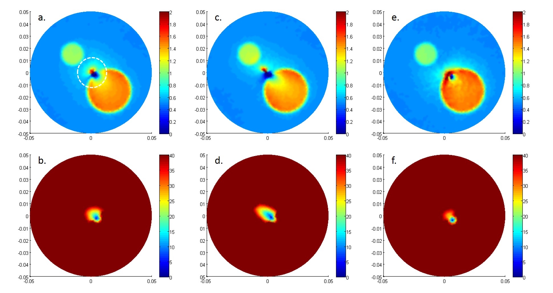
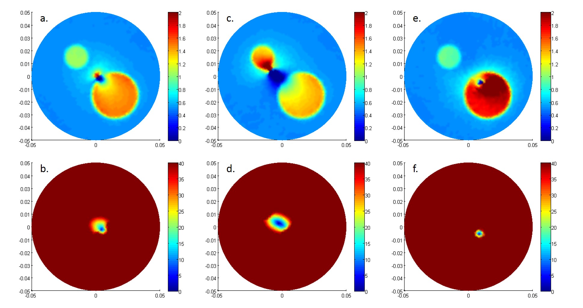
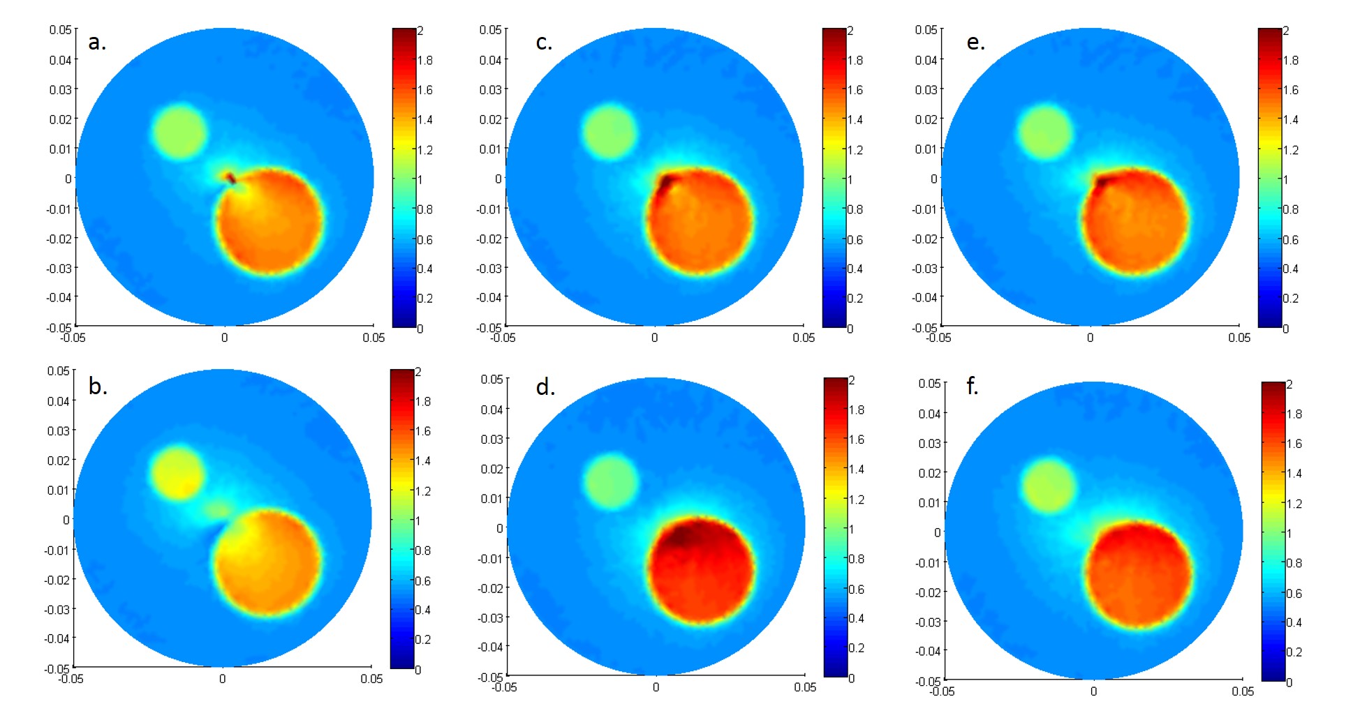
Figure 4: Combined conductivity maps a. No pad and left-side $$$\epsilon_{r}$$$= 80 pad. b. No pad and left-side $$$\epsilon_{r}$$$= 350 pad c. No pad and right-side $$$\epsilon_{r}$$$= 80 pad d. No pad and right-side $$$\epsilon_{r}$$$= 350 pad. e. Left and right-side $$$\epsilon_{r}$$$= 80 pad, d. Left and right-side $$$\epsilon_{r}$$$= 350 pad, the conductivity values of anomaly regions for this combination are similar to original values.