1948
Three-Dimensional Model-Based Conductivity Mapping with Regularization and a Non-Negativity Constraint1Biomedical Engineering, University of Michigan, Ann Arbor, MI, United States
Synopsis
We present a three-dimensional model-based approach to calculating conductivity using MRI. Our proposed method is formulated as an inverse problem based on the phase-based conductivity equation. The algorithm includes an edge-preserving regularization term and we explore the utility of non-negativity constraints. Structural information is also used to inform regions over which to regularize. We present results for simulation, phantom, and human brain data.
Purpose
To develop a three-dimensional model-based conductivity mapping algorithm that improves the accuracy and reduces noise in conductivity maps.Methods
The proposed Inverse Laplacian (IL) method is based on the phase-based approximation to conductivity,
$$\sigma\approx\frac{\nabla^2 \phi^+}{\omega \mu_0}$$
where σ is conductivity, φ+ is the phase of the transmit RF field, ω is the resonant frequency of the MRI scanner, and µ0 is the permeability of free space1,2. Our proposed estimator of the conductivity map is
$$\widehat{\boldsymbol\sigma}=argmin_{\sigma}\frac{1}{2}||\frac{\boldsymbol\phi^+}{\omega\mu_0}-\boldsymbol L\boldsymbol\sigma||_{\boldsymbol{W_1}}^{2}+\beta{\boldsymbol{W_2}}{R}(\boldsymbol\sigma)$$
where $$$\hat{\boldsymbol\sigma}$$$ is the optimal conductivity map, L is the model relating the measured transmit phase (φ+) and the conductivity, R is a regularization function, and β is the regularization parameter3 . W1 is a binary mask defining the region of support for the problem, derived from a magnitude image. W2 is a binary mask that is zero-valued at object edges, identified from a magnitude image, so that regularization is only enforced in regions of relatively constant magnitude, under the assumption that large changes in conductivity will coincide with large changes in magnitude.
The IL model, L, is a filter calculated by inverting the Discrete Fourier Transform coefficients of the 3D Laplacian operator. A small offset on the order of 10-3 was added to the DC coefficient of the Laplacian operator to prevent division by zero. The IL filter is applied in the frequency domain: $$$\boldsymbol L \boldsymbol\sigma=\it F^{-1}\tt\left\{\it F\tt\left\{\boldsymbol\sigma\right\}\cdot\it F\tt\left\{\boldsymbol L\right\}\right\}$$$.
The regularizer used in this problem is based on the 3D finite differences operator. We used the hyperbola form of potential function, which has edge-preserving qualities while remaining differentiable4.
We explored the use of a non-negativity constraint, which was implemented by hard thresholding negative values to zero after each iteration of the optimization problem in the second equation. In contrast to setting all negative values of the final solution to zero, this produces smoother conductivity maps.
For comparison, we also implemented a restricted filtering approach, where conductivity was calculated directly using the first equation, then the results filtered using a 5x5x5 Gaussian filter with standard deviation of 1 pixel. The filtering was restricted based on the magnitude data such that only voxels with intensities within 20% of the center voxel were included. After filtering, all negative values were set to zero.
We present results for simulation, phantom, and human brain data. Simulations were performed using SEMCADX using 0.4 mm3 isotropic voxels. Phantom and human subject data were acquired on a GE 3.0T MRI scanner with a birdcage head coil using a 2D spin echo sequence, repeated twice with opposite slice select gradient polarity and averaged. Scan parameters were: TE/TR = 16/1200 ms, FOV = 24x24x2.1 cm, 1.25x1.25x3.0 mm3 voxels. Transmit phase was calculated as half of the phase of the spin echo image. Four volunteer subjects were scanned under IRB approval.
Results
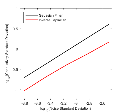
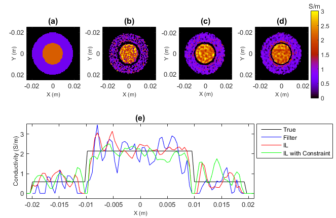
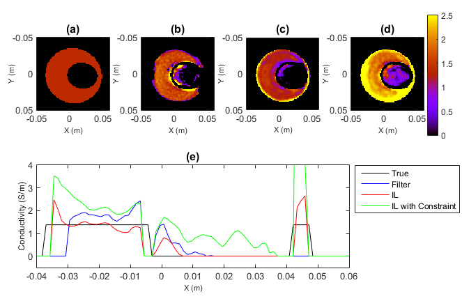
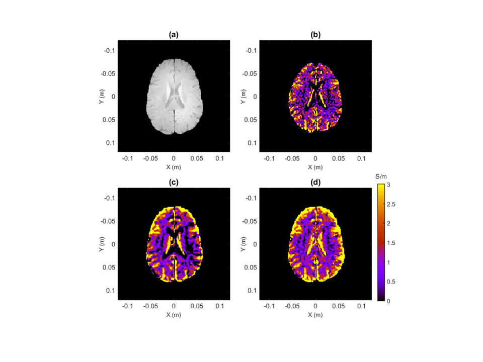
The IL method results in lower standard deviations in conductivity maps than the Gaussian filter method for a given input noise level, as shown in Figure 1. Simulation results in Figure 2 show that the IL method reduces the width of the edge artifact between compartments as compared to the filter. The non-negativity constraint slightly elevates the conductivity values near the compartment boundary. Phantom results, shown in Figure 3, show that the IL method produces more accurate conductivity values with lower standard deviation, but adding the non-negativity constraint elevates the average conductivity values in both compartments. Figure 4 shows the conductivity maps from a representative human brain. We note that the white matter conductivity values are more uniform with the IL method (0.54$$$\pm$$$0.42 S/m) than the filtering method (0.65$$$\pm$$$0.54 S/m), and further improved by using the non-negativity constraint (0.76$$$\pm$$$0.41 S/m). By visual inspection, the constraint does not noticeably elevate the peak tissue conductivity values as in the phantom, but the difference in white matter mean values can be attributed to the reduction of zero-valued voxels.Discussion
When applying a spatial filter to conductivity maps, there is typically a trade-off between spatial resolution and SNR. With the IL method we reduce noise levels without a loss of small object features. The non-negativity constraint is motivated by the fact that conductivity cannot be negative. This constraint reduces the standard deviation of conductivity maps, but caused elevated average conductivity values in the phantom.Conclusions
We have presented a three-dimensional model-based method for conductivity mapping with regularization. The proposed IL method is more robust to high noise levels in transmit phase data, which is important for high resolution imaging. Additionally, the non-negativity constraint decreases the standard deviation of conductivity values.Acknowledgements
No acknowledgement found.References
[1] Katscher U, Voigt T, Findeklee C, Vernickel P, Nehrke K, Dossel O. Determination of conductivity and local SAR via B1 mapping. IEEE Trans Med Imag 2009;28:1365-1374.
[2] Wen H. Non-invasive quantitative mapping of conductivity and dielectric distributions using the RF wave propagation effects in high field MRI. In Prceedings of SPIE 5030, Medical Imaging 2003: Physics of Medical Imaging, San Diego, CA, USA, 2003. pp. 471-477.
[3] Ropella KM, Noll DC. A Regularized Model-Based Approach to Phase-Based Conductivity Mapping. In Proceedings of the 23rd Annual Meeting of the ISMRM, Toronto, ON, Canada, 2015. pp. 3295.
[4] Panin VY, Zeng GL, Gullberg GT. Total variation regulated EM algorithm. IEEE Trans Nucl Sci 1999;46:2202-2210.
Figures