1937
Quantitative relaxation time mapping of axillary lymph nodes and recommended parameters for 3T lymphatic node substructure imaging1Radiology and Radiological Sciences, Vanderbilt University Medical Center, Nashville, TN, United States, 2Physical Medicine and Rehabilitation, Vanderbilt University Medical Center, Nashville, TN, United States, 3Vanderbilt Dayani Center for Health and Wellness, Nashville, TN, United States, 4Neurology, Vanderbilt University Medical Center, Nashville, TN, United States, 5Psychiatry, Vanderbilt University Medical Center, Nashville, TN, United States, 6Physics and Astronomy, Vanderbilt University, Nashville, TN, United States
Synopsis
A lack of MRI methods exist that are designed with sensitivity to the lymphatics, even though components of the lymphatic system have been discovered in every major organ system of the body and likely play an understudied role in disease. In this work we performed quantitative relaxation time mapping in axillary lymph node substructures, the cortex and hilum, for the first time at 3 Tesla and used these values to optimize structural imaging parameters for the lymphatics. Knowledge of fundamental MR parameters in the lymphatics is the first step to developing novel imaging sequences that exploit lymphatic tissue in vivo.
Purpose
The goal of this work is to quantify 3T MRI relaxation times in vivo in human axillary lymphatic nodes for the first time, which will enable the development of optimized structural and functional imaging protocols for evaluating lymph node morphology and function in patients with breast cancer and related co-morbidities. More specifically, metastatic lymph nodes can become inflated with focal MR hyper/hypointensities in the cortex and may be devoid of a hilum1. However, MRI is not used routinely for lymph node imaging and there is a lack of knowledge of even the most fundamental MRI parameters, e.g., T1 and T2 relaxation time, of healthy lymph node substructures. Additionally, more novel MRI methods, such as CEST2 and spin labeling3 are being applied for lymphatic imaging, however the quantitative accuracy of these methods is suboptimal without knowledge of lymph relaxation times. Here, we quantify lymphatic node substructure relaxation times for the first time at 3T, and use this information to recommend optimal imaging protocols for lymph node imaging using MRI.Methods
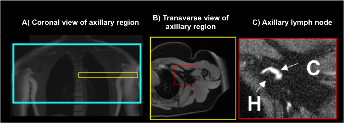
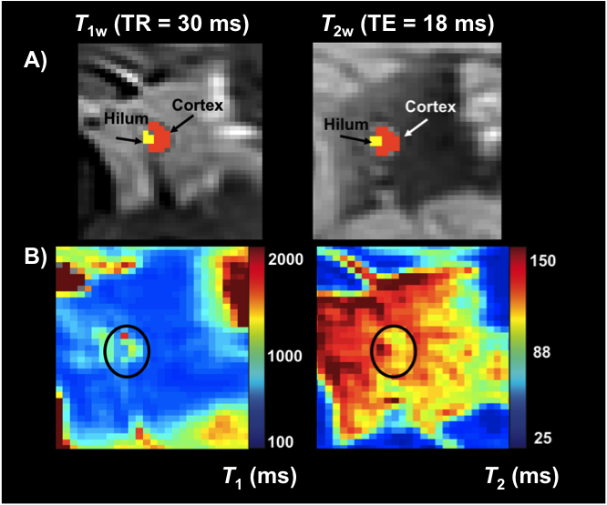
Healthy females (n=15; age=45±13 years; body-mass-index=28.7±7.8kg/m2) were imaged supine using a torso coil (16-channel RX) at 3T (Philips Achieva). The axillary region was located (Figure 1A) and axillary lymph nodes identified on transverse images acquired with the multi-point Dixon method to produce water-only (Figure 1B) and fat-only contrast with the following parameters: TR=3.5ms, TE1=1.15ms, TE2=2.3ms; 3D gradient-echo; FOV=520x424x192mm3; spatial-resolution=0.9x0.7x2.5mm3; duration=18s). Sub-nodal structures of the cortex and hilum were visualized at high spatial-resolution by T2-weighted imaging with fat suppression (SPAIR) using: TR/TE=3500/60ms; FOV=180x180x50mm3; resolution=0.3x0.3x5mm3; Figure 1C). Quantitative relaxation time mapping was performed over a bilateral FOV (520x424x49.5mm3; slices=9, spatial-resolution=1.80x1.47x5.5mm3). T2 mapping was achieved using TE=9–189ms (interval=12ms), and TR=4000ms. T1 mapping was achieved using the mutli-flip angle method (FA=20, 40, 60 degrees, TR/TE=100/4.6ms)4. Flip angle inefficiency was corrected using a B1 map acquired by a dual-TR approach (TR1=30ms, TR2=130ms, FA=60 degrees). Relaxation time maps and B1-efficiency correction were calculated using custom routines in Matlab and previously published algorithms2. Segmentation of the nodal cortex was carried out manually (Figure 2) in 40 lymph nodes and a discernable fatty hilum region was segmented in 34 of these nodes. Surrounding tissue regions were segmented from the arm muscle and periscapular fat tissue. Finally, protocols for optimal lymph node substructure contrasts were evaluated experimentally for T1-weighted and T2-weighted imaging.Results
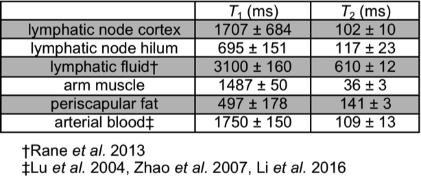
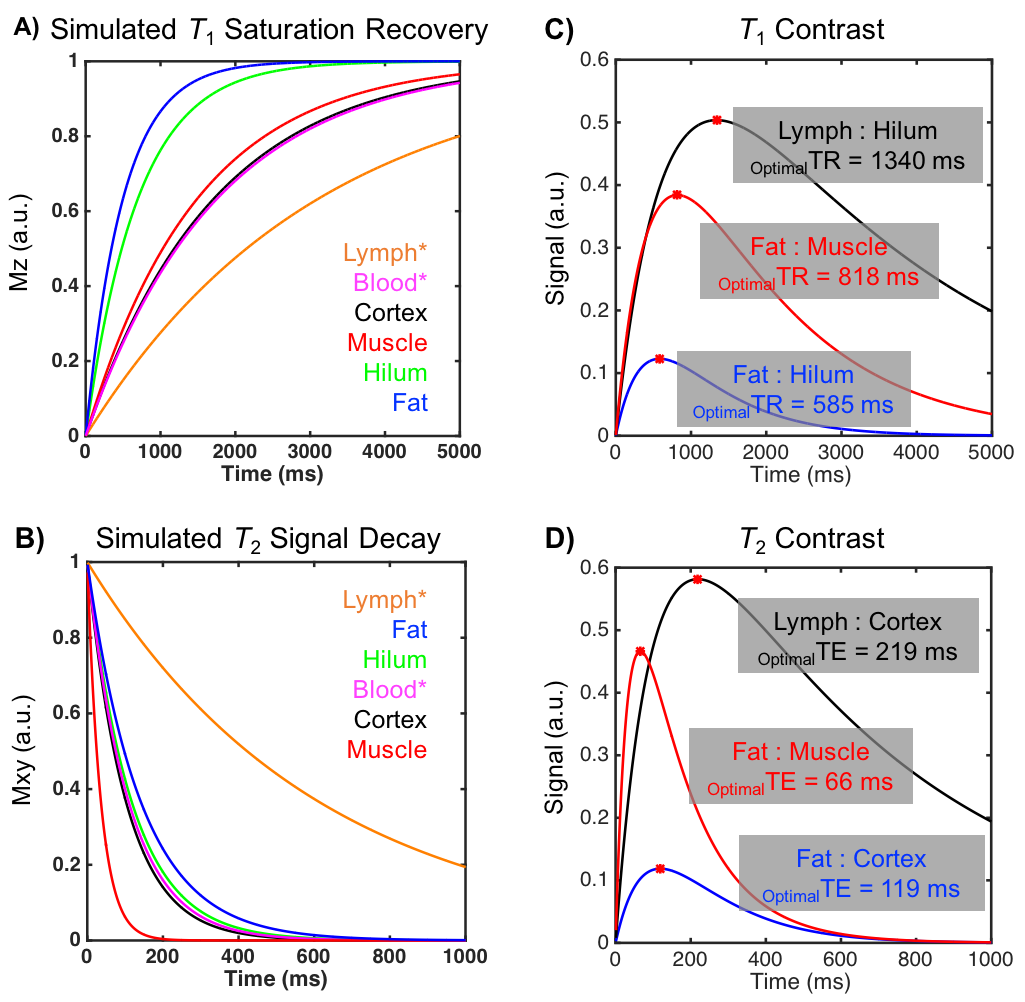
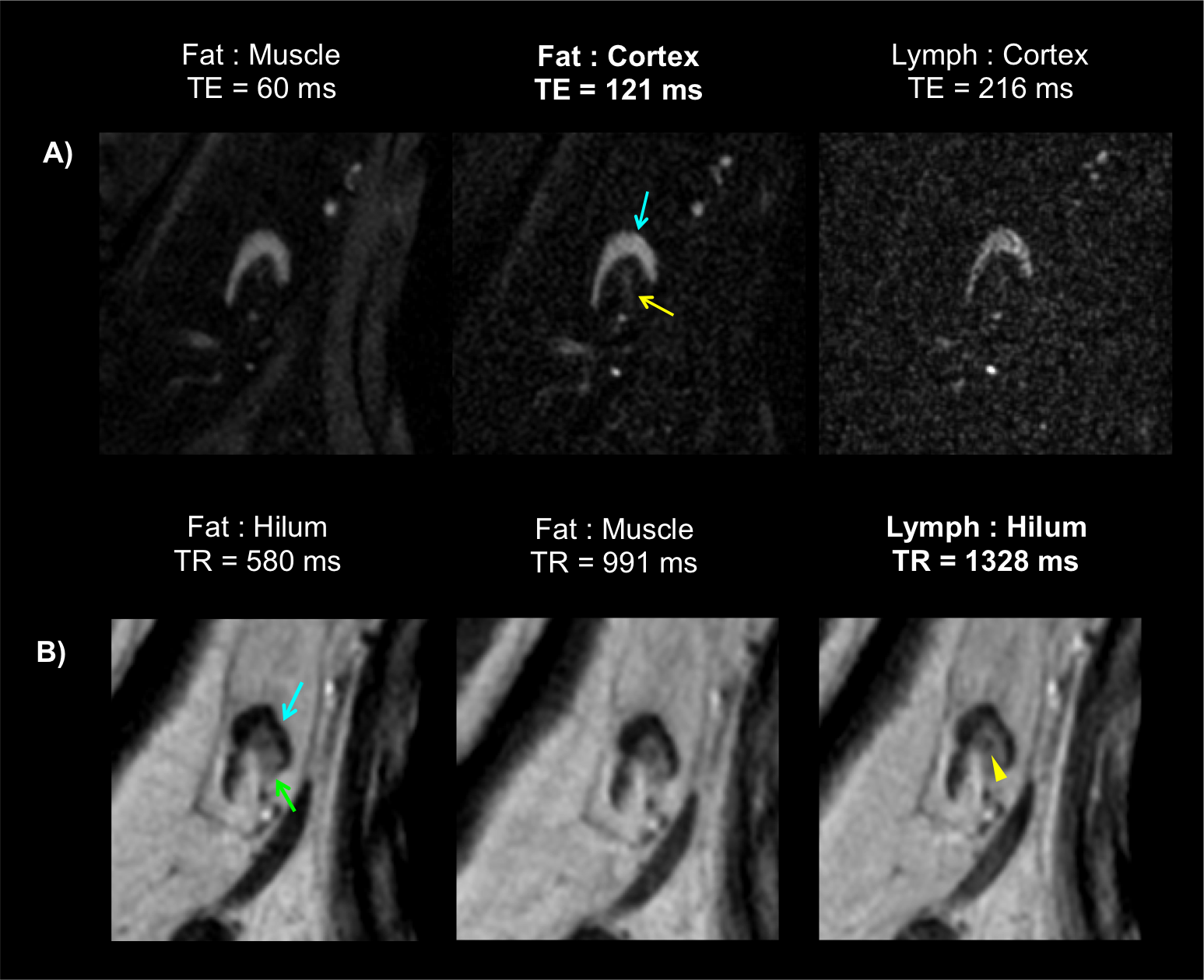
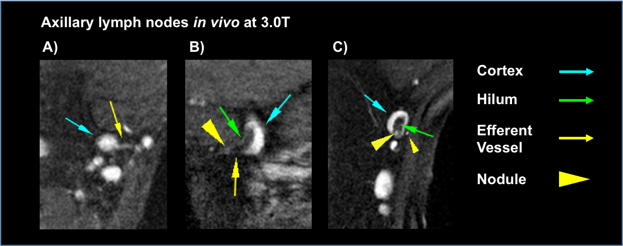
Table 1 reports measured T1 and T2 values of lymphatic structures and tissues inferior to axilla, in addition to literature values of measured relaxation times in lymphatic fluid3 and arterial blood5-6. Figure 3A-B reports the simulated longitudinal signal (Mz) recovery or transverse signal (Mxy) decay of these tissues, and Figure 3C-D reports the difference in signal between tissues of interest, where the maximum difference indicates the optimal TR or TE to achieve image contrast. Figure 4A shows that optimized contrast between the cortex of a lymph node and surrounding axillary fat on a T2-SPAIR acquisition was achieved at TR/TE=3500/121ms. Additionally a lymphatic vessel can be visualized at TE=121ms compared to shorter or longer TEs sampled. Using a T1-weighted acquisition, the hilum of a lymph node exhibits optimal contrast from the cortex at TR=580ms. Within the hilum a hypointensity is discerned at TR=1328ms, in accord with TR optimized between lymphatic fluid and hilum (Figure 4B). Visualization of lymph node substructures and efferent vessels was achieved at high spatial resolution in vivo at 3T (Figure 5).Discussion
Based on relaxation time parameters measured here in healthy lymphatic tissue at 3T, we propose a structural imaging protocol which offers improved spatial resolution and identification of lymphatic tissue including nodes and vascular architecture: T2-weighted TR/TE=3500/121ms; and T1-weighted TR/TE=1328/15ms. Hypointesities, like that observed in Figure 4B in vivo, were also observed in excised lymph nodes imaged at 7T that correlated with activated B-cell follicles on pathology7. These heterogeneous features likely contribute to a higher standard deviation of T2 values measured here in the hilum. Optimal contrast within the cortex and hilum may be desirable for determining tumor perimeter as a marker of response to neoadjuvant therapy8. Further, evaluation of the density of lymphatic microvasculature may allow detection of lymphangiogenesis9, which may be protective in certain cancers10.Conclusion
These methods allow for improved clinical imaging of lymph node structure without the use of exogenous contrast agents, using protocols that can be implemented in less than five minutes with coverage of the entire axilla. Measurement of T1 and T2 relaxation time constants in lymphatic tissue should have relevance for developing novel MR imaging and angiography techniques with sensitivity to lymphatic physiology.Acknowledgements
No acknowledgement found.References
1. Memarsadeghi M, Riedl C, Kaneider A, et al. Axillary Lymph Node Metastases in Patients with Breast Carcinomas: Assessment with Nonenhanced versus USPIO-enhanced MR Imaging. Radiology. 2006;241(2):367-377.
2. Donahue MJ, Donahue PC, Rane S, et al. Assessment of lymphatic impairment and interstitial protein accumulation in patients with breast cancer treatment-related lymphedema using CEST MRI. Magnetic Resonance in Medicine. 2015;75(1):345-355.
3. Rane S, Donahue PMC, Towse T, et al. Clinical feasibility of noninvasive visualization of lymphatic flow with principles of spin labeling MR imaging: implications for lymphedema assessment. Radiology. 2013;269(3):893-902.
4. Wang J, Qiu M, Kim H, et al. T1 Measurements incorporating flip angle calibration and correction in vivo. Journal of Magnetic Resonance. 2006;182(2):283-292.
5. Zhao JM, Clingman CS, Narvainen MJ, et al. Oxygenation and hematocrit dependence of transverse relaxation rates of blood at 3T. Magnetic Resonance in Medicine. 2007;58(3):592-597.
6. Li W, Grgac K, Huang A, et al. Quantitative theory for the longitudinal relaxation time of blood water. Magnetic Resonance in Medicine. 2016;76(1):270-281.
7. Korteweg MA, Zwanenburg JJM, van Diest PJ, et al. Characterization of ex vivo healthy human axillary lymph nodes with high resolution 7 Tesla MRI. European Radiology. 2011;21(2):310-317.
8. Liu SV, Melstrom L, Yao K, et al. Neoadjuvant therapy for breast cancer. Journal of Surgical Oncology, 2010;101(4):283-291.
9. Alitalo K, Tammela T, Petrova TV. Lymphangiogenesis in development and human disease. Nature. 2005;438(7070):946-953.
10. Fischbein NJ, Noworolski SM, Henry RG, et al. Assessment of metastatic cervical adenopathy using dynamic contrast-enhanced MR imaging. American Journal of Neuroradiology. 2003;24(3):301-311.
Figures