Synopsis

A method for noninvasive assessment of mouse glomerular filtration rate (GFR) using dynamic contrast enhanced MRI (DCE-MRI) was developed and validated. The kinetics of gadolinium in the abdominal aorta and two kidneys were measured using a snapshot fast low angle shot based T₁ mapping method with a temporal resolution of 1 s. A modified bi-compartmental model was used for quantification of GFR by a least-squares fitting. As a reference standard, GFR was also measured using FITC-inulin clearance. Single-kidney GFR measured from both methods showed a good agreement, suggesting the proposed DCE-MRI method provides an accurate measurement of murine single-kidney GFR.

Introduction

Methods

DCE-MRI Study. This study was approved by the Institutional Animal Care and Use Committee. MRI studies were performed on a vertical 16.4 T Bruker scanner equipped with a 38-mm inner diameter birdcage coil. Seven male 129S1 mice 4 weeks after either unilateral sham (n=4) or renal artery stenosis (RAS, n=3) surgeries were used. A saturation recovery T₁ mapping method with snapshot fast low angle shot readout was developed to trace Gd dynamics with a temporal resolution of 1 s. Two slices located at the center of both kidneys were imaged. Following acquisition of the proton density (M₀) and ten baseline T₁-weighted (M_t) images, 37.5 mM gadodiamide (0.03mmol/kg) was injected through the tail-vein within 2 s, after which the M_t images were acquired repetitively. Other imaging parameters were: recovery time, 0.25 and 0.57 s; encoding scheme, central; TR 4.92 ms; TE 0.8 ms; flip angle 15°; slice thickness 2 mm; FOV 2.56×2.56 cm²; matrix size 128×128; number of repetitions 150. T₁ maps were generated by mono-exponential fitting and the change in R₁ (ΔR₁) from baseline was used as an index of Gd concentration.

In addition, kidney volume was measured using a three-dimensional fast imaging with steady precession sequence, and renal perfusion using a flow-sensitive alternating inversion-recovery sequence with rapid acquisition with relaxation enhancement, as described previsouly³.

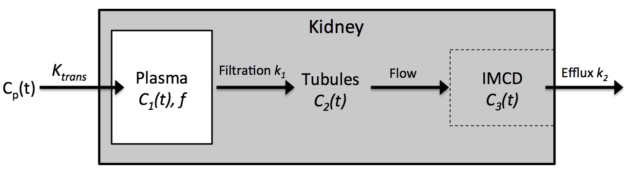
Compartmental Model. The compartmental model is shown in Fig. 1. The kidney is compartmentalized into plasma and tubules. In this model, C₁(t) is the Gd concentrations in renal plasma and C₂(t) is the Gd concentration in the tubules within the whole kidney. Changes in C₁(t) and C₂(t) can be described by the following kinetic equations:

dC₁(t)/dt=K_trans(C_p(t)-C₁(t))

dC₂(t)/dt=k₁C₁(t)-k₂C₃(t)

where K_trans is the perfusion rate constant, C_p(t) the arterial input function (AIF), k₁ the normalized GFR, k₂ the Gd efflux rate, and C₃(t) the concentration of filtered Gd in the inner medullary collecting ducts (IMCD) space. In image analysis, the IMCD space was prescribed at the innermost part of medulla that did not show the blooming effect of Gd. The total Gd concentration in kidney is C(t)=C₁(t)×f+C₂(t), where f is the volume fraction of renal plasma space. Dynamic curves were model-fitted with the Levenberg-Marquardt least-squares algorithm. Then GFR (ml/min) was calculated as k₁×V×60, where V is the effective kidney volume.

GFR by FITC-inulin Clearance. One day after MRI, GFRs of the same mice were measured by FITC-inulin clearance⁴. 3.5% FITC-inulin 3.74 ml/g was injected retro-orbitally, after which ~20ml blood was repeatedly collected via the saphenous vein at 3, 7, 10, 15, 35, 55, and 75 minutes. The concentration of FITC-inulin in isolated plasma was measured using fluorescence, with 485 nm excitation and 538 nm emission. A two-compartment model was used, in which the concentration of FITC-inulin was described by A×e^-at + B×e^-bt, with the first and second term represents redistribution and clearance, respectively. GFR was then calculated as I/(A/a+B/b), where I is the total amount of injected FITC-inulin. Single-kidney GFR was quantified by partitioning the total GFR based on the blood flow (perfusion × volume) of each kidney.

Results

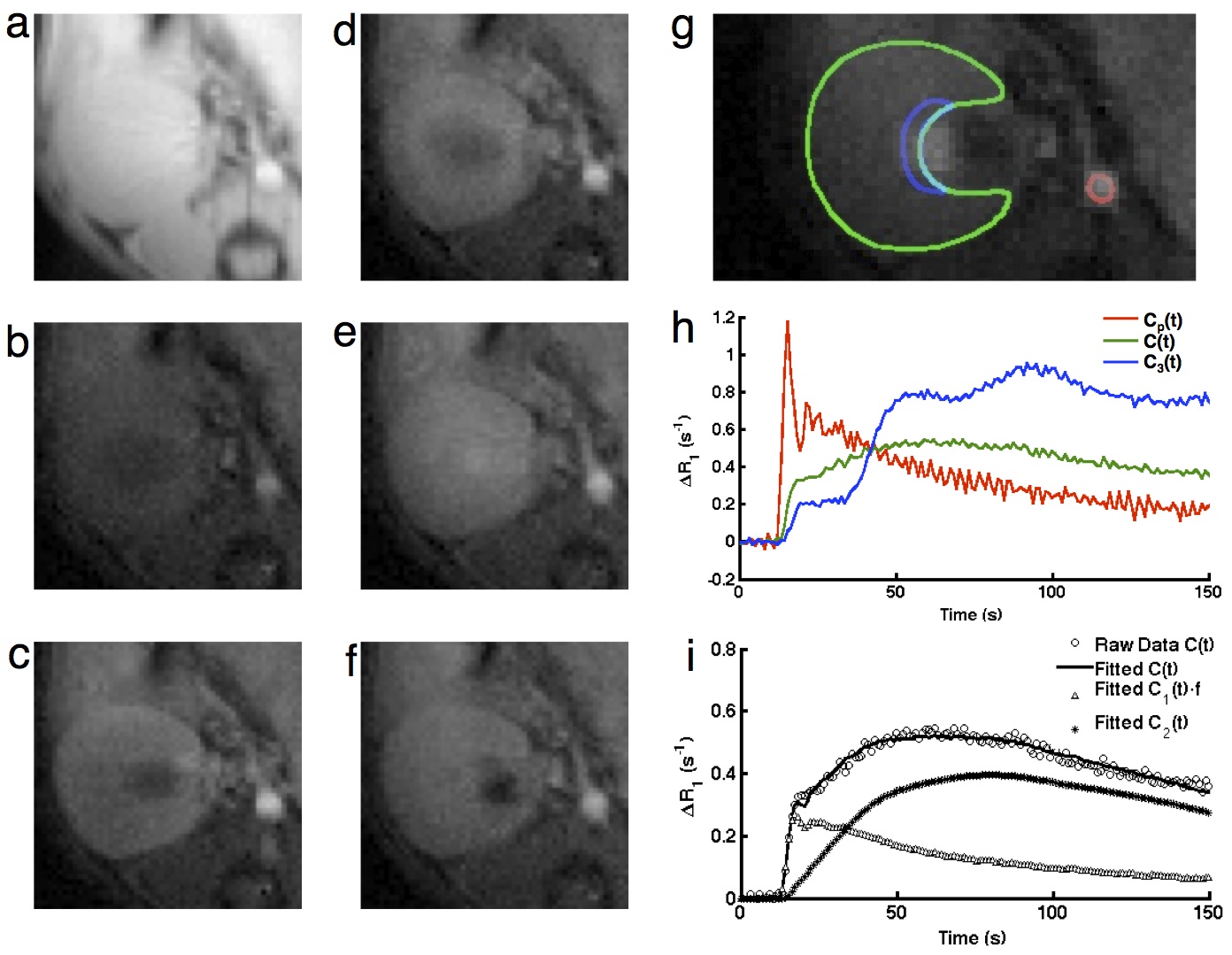
Fig. 2 a-f shows representative M₀ (Fig. 2a) and M_t images acquired at baseline (Fig. 2b) and 5, 17, 73, and 138 s post-Gd injection (Fig. 2c-f). Manually traced regions of interest (ROIs) for the abdominal aorta (red), kidney (green), and IMCD (blue) are shown in Fig. 2g. The corresponding time-intensity curves of Gd concentration in all three ROIs are shown in Fig. 2h, and the model-fitted curves in Fig. 2i.

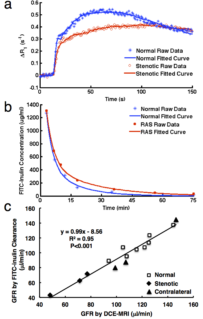
Representative raw data and model-fitted Gd dynamics in normal and stenotic kidney are shown in Fig. 3a. The attenuated stenotic kidney curve suggests impaired perfusion and filtration, which was also reflected in the slower clearance of FITC-inulin from plasma (Fig. 3b). A good correlation was found between GFRs measured by DCE-MRI and FITC-inulin clearance of normal, stenotic, and contra-lateral kidneys (Fig. 3c).

Conclusion

Acknowledgements

References

1. Lee VS, Rusinek H, Bokacheva L, et al. Renal function measurements from MR renography and a simplified multicompartmental model. Am. J. Physiol. Renal Physiol. 2007;292:F1548–F1559.

2. Annet L, Hermoye L, Peeters F, Jamar F, Dehoux J-P, Van Beers BE. Glomerular filtration rate: assessment with dynamic contrast-enhanced MRI and a cortical-compartment model in the rabbit kidney. J. Magn. Reson. Imaging 2004;20:843–9.

3. Jiang K, Ferguson CM, Ebrahimi B et al. Noninvasive Assessment of Renal Fibrosis with Magnetization Transfer MR Imaging: Validation and Evaluation in Murine Renal Artery Stenosis. Radiology, 2016, Ahead of Print, 10.1148/radiol.2016160566

4. Qi Z, Whitt I, Mehta A, et al. Serial determination of glomerular filtration rate in conscious mice using FITC-inulin clearance. Am J Physiol Renal Physiol. 2004;286(3):F590-6.