1910
Influence of parameter initial values on DCE parameter estimates in pharmacokinetic modeling: a simulation study1German Cancer Consortium (DKTK), Heidelberg, Germany, 2Translational Radiation Oncology, Heidelberg Institute of Radiation Oncology (HIRO), German Cancer Research Center (DKFZ), Heidelberg, Germany, 3Department of Radiation Oncology, Heidelberg Ion-Beam Therapy Center (HIT), Heidelberg University Hospital, Heidelberg, Germany, 4National Center for Tumor Diseases (NCT), Heidelberg, Germany, 5Software development for Integrated Diagnostics and Therapy, German Cancer Research Center DKFZ, 6Institute for Clinical Radiology, Ludwig-Maximilians-University Hospital Munich
Synopsis
In pharmacokinetic analysis of DCE-MRI data, the choice of initial parameter values for fitting has been reported to have a significant impact on the outcome of the optimization and hence, on parameter estimates. In this study, we investigated the influence of initial values by fitting simulated concentration time curves with varying combinations of initial parameters, using the two compartment exchange model. The resulting parameter estimates were visualized and compared to the true values, used for simulation, by means of relative errors. Results showed that the choice of initial values has little influence on the precision of the pharmacokinetic analysis.
Purpose
Parameter estimation in dynamic
contrast-enhanced MRI is usually performed by fitting a
pharmacokinetic model to the measured data, using non-linear least
square methods.
The two-compartment exchange model (2CXM) describes the compartments
„plasma“ and „interstitial volume“ with fractional volumes vp
and ve,
and their exchange in terms of plasma flow Fp
and permeability-surface area product PS1,2.
The choice of initial parameter values for fitting
can influence the analysis outcome. In the presence of several local
minima of the costfunction, the optimizer starting position will
determine the direction of search.
This effect has been mentioned3
and authors have put forth considerable efforts to compensate it by using
time-consuming variations of initial values4.
We studied the influence of
different starting values on precision and accuracy of parameter
estimates in the 2CXM.Methods
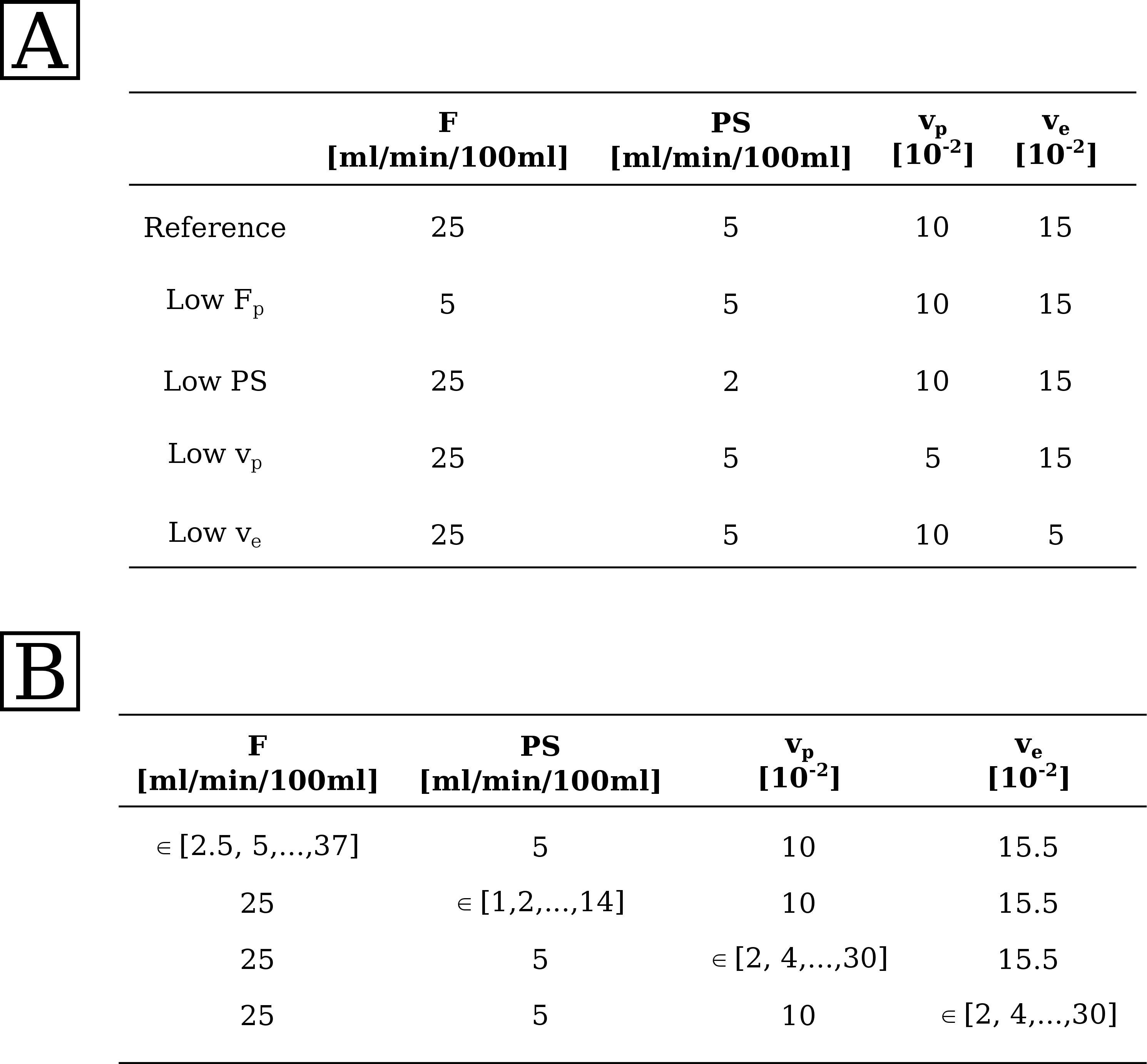
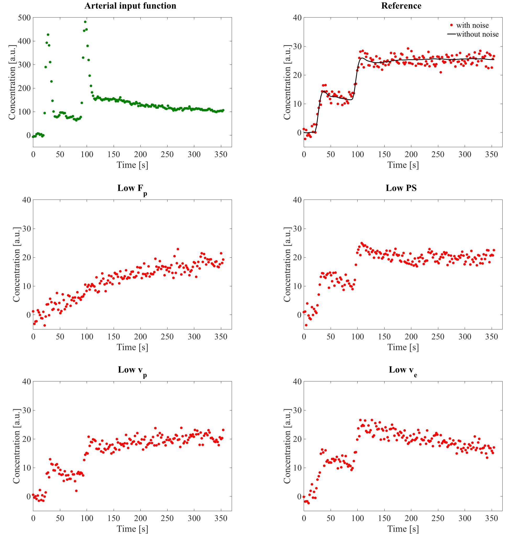
Five types of tissue curves, defined by specific combinations of perfusion parameters (figure 1, table A), were used to simulate time-resolved concentration images of 15x60 px by convolution of a measured arterial input function (temporal resolution 2.11s, 169 timepoints5) with 2CXM tissue response functions. To account for acquisition noise, Gaussian random numbers were added to each data point. Standard deviation of the noise was chosen to achieve a contrast-to-noise ratio (CNR) of 300. CNR is defined as the ratio between AIF peak and standard deviation of the noise.
All curves were fitted with the 2CXM, using an
in-house written software module6, implemented in the Medical Imaging Interaction Toolkit7.
This tool allows definition of initial optimization values for each
parameter on a pixelwise basis, which opens the possibility to use
various combinations of initial parameters and graphically visualize
the resulting parameter estimates.
Parameter constraints were applied to assure
model consistency : $$$ 0<v_{p},v_{e}<
1,\: v_{p}+v_{e}<1,\:
0<F_{p}<100\: [ml/min/100ml], \:-1<PS< 100\: [ml/min/100ml] $$$. Initial parameter values were
defined in 15x60 px images, with one parameter varying along the
x-axis and the other three kept fixed (figure 1, table B). Parameter
estimates were averaged over all 60 px with the same set of initial
values.
Accuracy
of the average parameter estimate of all four model parameters $$$\bar{P}_{fit}$$$
was evalutated by means of the relative error with respect to the simulation input
values $$$P_{input}$$$:
$$E_{rel}= \frac{\bar{P}_{fit} - P_{input}}{P_{input}}$$
Results
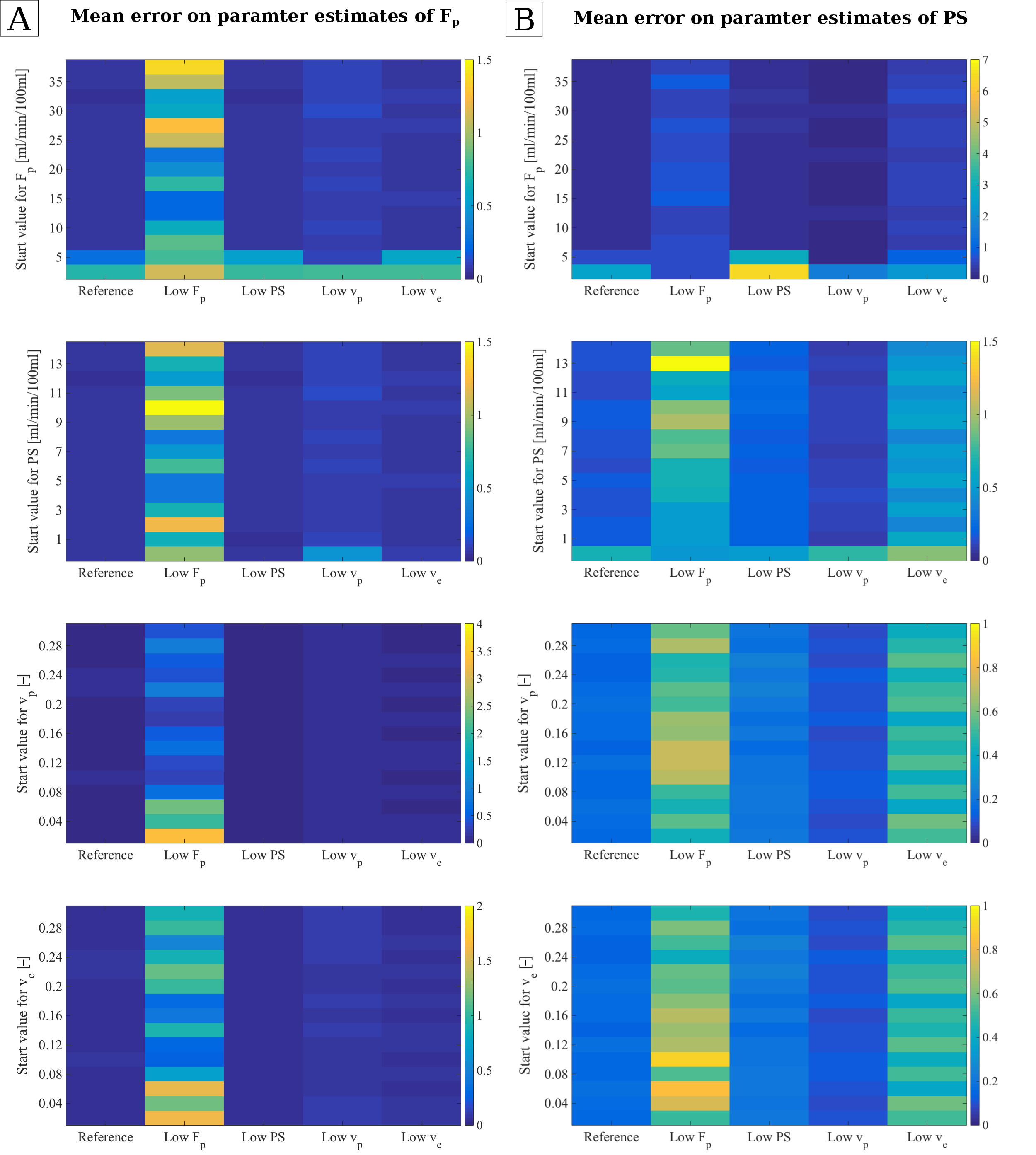
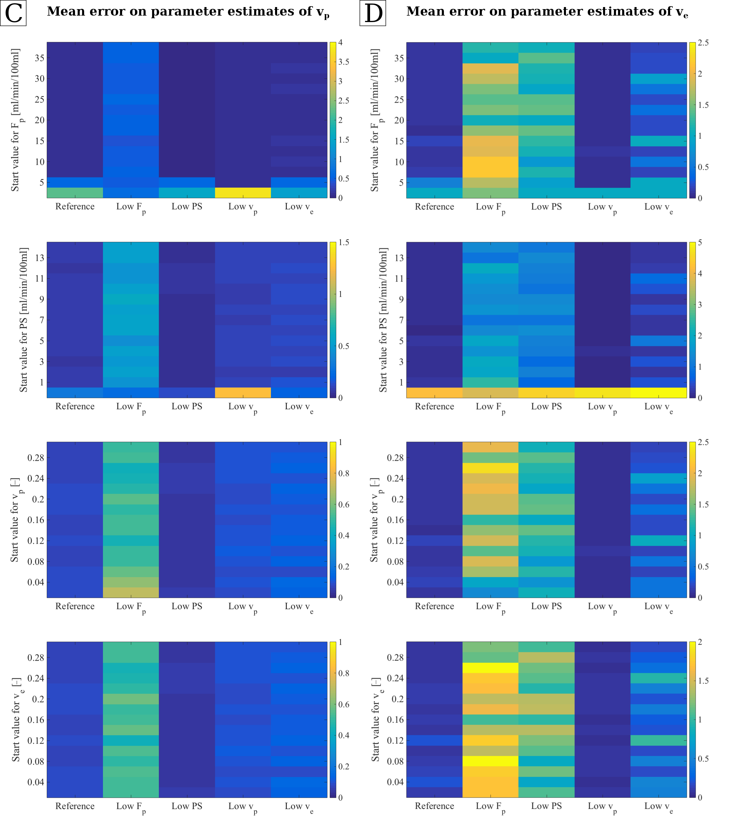
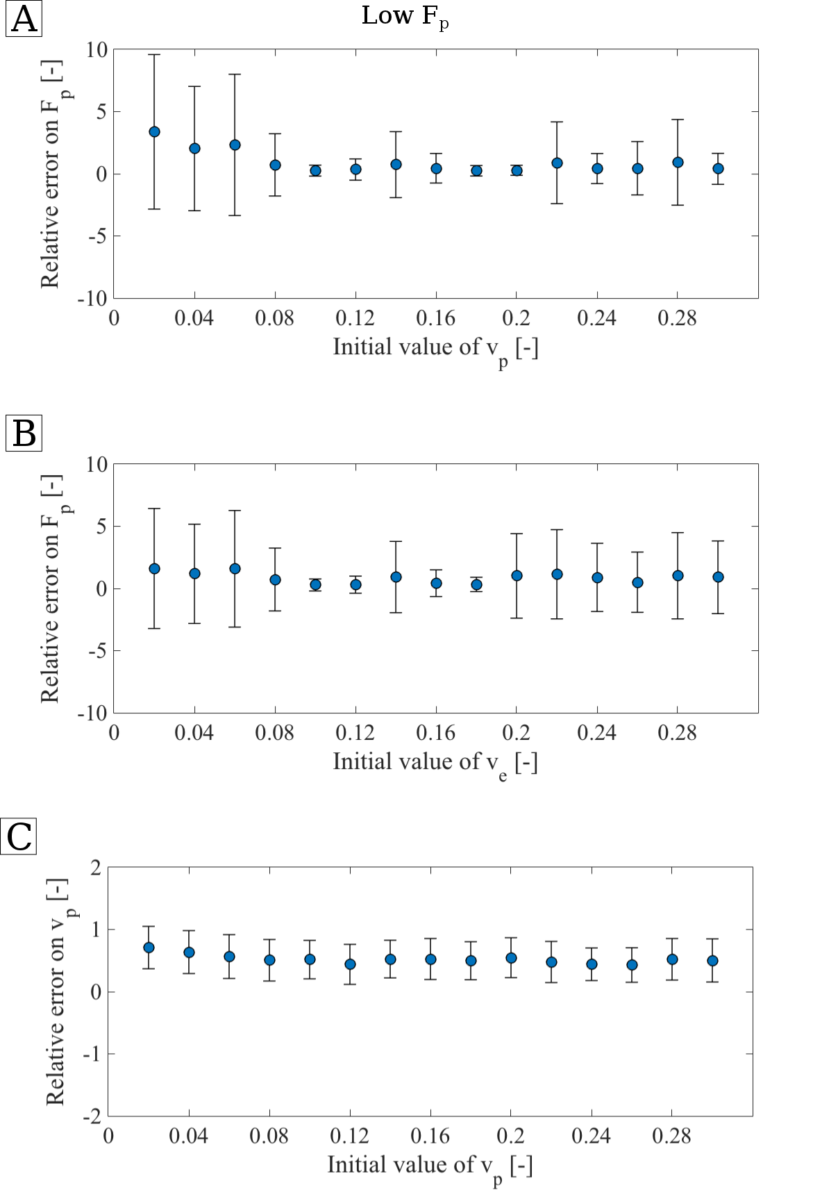
Figure 3 illustrates relative errors on parameter estimates of Fp(A) and PS(B) for the five different curve types (x-axis), fitted with each one parameters' initial value varying as indicated on the y-axis. The errors on parameter estimates on vp(C) and ve(D) are mapped in the same manner in figure 4. Parameter estimates for Fp show low errors, except for low Fp curves. The error is increased in all curve types fitted with low initial values of Fp. For low Fp curves, the estimates on Fp seem to correlate with starting value of vp and ve. For further investigation, the mean errors on Fp is plotted over the initial value of vp and ve in figure 5 A and B. Within the standard deviation, the parameter estimates show no correlation with the initial values. Errors on PS were higher, compared to Fp, and increased for low initial values of Fp and PS. Curves with low Fp or low ve showed higher errors on the estimate for PS. Estimates of vp had low errors, except for curve with low Fp. Errors were increased for inital values Fp=2.5 ml/min/100ml and PS=2.5 ml/min/100ml. For curve types with low Fp, the estimate on vp seems to correlate with the initial value of vp, especially at low starting values. Figure 5C shows the mean error on vp for curves with low plasma flow over the varying initial value of vp. No correlation is visible within the standard deviation. Errors on ve showed the highest errors of all estimates, especially for low Fp and low PS curves. The errors were distinctively larger if the start value for PS was set to 0. Apart from this, no correlation with the initial parameter values can be seen.Conclusion
The influence of starting values of the optimization routine on the accuracy of the initial parameters is less than expected. Estimates on Fp and PS are sensitive to their own start values if chosen too low. Apart from that, no further correlation between initial value and error on the estimate could be found. Results indicate that time-consuming searches over the initial parameter grid are not necessary, as the effects succumb those generally occuring in pharmacokinetic modeling. However, we investigated the effects of varying one initial parameter. For further clarification, the next step would be to vary initial values for two parameters simultaneously.Acknowledgements
No acknowledgement found.References
1 Sourbron, S. P., and Buckley, D. L. "Tracer kinetic modelling in MRI: estimating perfusion and capillary permeability." Physics in medicine and biology 57.2 (2012): R1.
2 Brix, Gunnar, et al. "Tracer kinetic modelling of tumour angiogenesis based on dynamic contrast-enhanced CT and MRI measurements." European journal of nuclear medicine and molecular imaging 37.1 (2010): 30-51
3 Brix, Gunnar, et al. "Pharmacokinetic analysis of tissue microcirculation using nested models: multimodel inference and parameter identifiability.", Medical Physics 36.7 (2009), 2923–2933
4 Buckley, David L. "Uncertainty in the analysis of tracer kinetics using dynamic contrast-enhanced T1-weighted MRI." Magnetic Resonance in Medicine 47.3 (2002): 601-606.
5 Ingrisch, Michael, et al. "Quantification of perfusion and permeability in multiple sclerosis: dynamic contrast-enhanced MRI in 3D at 3T." Investigative radiology 47.4 (2012): 252-258.
6 Debus, Charlotte et al „Impact of fitting strategy on DCE parameter estimates and performance : a simulation study in image space“, 24rd Annual meeting of the International Society of Magnetic Resonance in Medicine (2016), Vol. 24, International Society of Magnetic Resonance in Medicine (ISMRM)
7 Wolf, Ivo, et al. "The medical imaging interaction toolkit (MITK): a toolkit facilitating the creation of interactive software by extending VTK and ITK." Medical Imaging (2004). International Society for Optics and Photonics.
Figures