1901
Joint DCE- and DSC-MRI processing using the Gradient correction model1Magnetic Resonance and Cryogenics, Institute of Scientific Instruments of the CAS, v. v. i., Brno, Czech Republic
Synopsis
The contribution presents a method for simultaneous processing of the DCE- and DSC-MRI perfusion data acquired using a multi-echo sequence. It is an extension of the sequential application of the so-called gradient correction model. In the sequential approach, relaxivity parameters are estimated from the DSC signal based on perfusion parameters calculated from the DCE signal. Here the perfusion and relaxivity parameters are estimated using an iterative alternating optimization strategy. The impact on accuracy and precision is tested on synthetic data. The results show that the suggested approach can yield a remarkable improvement, especially for noisy data.
Purpose
DCE and DSC-MRI signals are usually acquired and processed separately, however, using multi-echo acquisition it is possible to acquire and process both signals simultaneously. As was shown before 1, simultaneously acquired DCE and DSC-MRI signals are processed sequentially. First, the DCE signal is processed using the two compartment exchange model (2CXM). The resulting perfusion parameters are then used in a gradient correction model (GCM - relates the DCE and DSC signals together) in processing of the DSC signal, which makes it possible to estimate two additional perfusion parameters of the GCM, the relaxivities r2vasc* and r2ees*. As was shown 2, the adiabatic approximation to tissue homogeneity (aaTH) model 3-5 is more reliable compared to the 2CXM in this scenario. However, any sequential processing of DCE and DSC-MRI can result in significant errors of r2vasc* and r2ees* estimates in case of errors in processing of the DCE signal. In this contribution, iterative alternating approximation of the DCE and DSC signals is proposed to avoid this drawback.Methods
The alternating approximation of the DCE and DSC signals is initialized by the sequential process, as described before 1, except for using the aaTH model instead of the 2CXM. The model is parametrized by plasma flow, (Fp[mL/min/mL]), extraction fraction (E[-]), extravascular-extracellular space (ve[mL/mL]), mean capillary transit time (Tc[min]) and the bolus arrival time (BAT[min]). The approximation task is implemented using the lsqnonlin function (MATLAB - The MathWorks, Inc. 6,7) with four initial guesses for DCE and three for DSC, which yields 12 unique initial solutions for the alternating approximation method. In evaluation, the initial solution with the minimal DCE fitting error is selected as the solution of the sequential approach.
The alternating approximation algorithm is run in 100 iterations. In each iteration, all perfusion parameters [Fp,E,ve,Tc,BAT,r2vasc*,r2ees*] are updated in the approximation of the DSC signal, and then [r2vasc*,r2ees*] are fixed and [Fp,E,ve,Tc,BAT] are updated in the approximation of the DCE signal. The process of 100 iterations is repeated for each of the 12 initial estimates and a set of parameters with a minimal DCE fitting error is the result.
For the comparison of the sequential and alternating approaches, a synthetic high temporal resolution (sampling period of 1s) data set with 600 time samples was generated. Tissue concentration curves were generated using the convolutional model with an analytical arterial input function (AIF) 8 and the aaTH impulse residue function, IRF(x), scaled by Fp. The IRFs parameters x=[Fp,E,ve,Tc,BAT] were set to [0.21,0.65,0.35,0.31,0.08] for a prostate tumor 9 and to [0.26,0.54,0.57,0.26,0.08] for a colorectal tumor 10 and finally to [0.05,0.16,0.08,0.20,0.08] for a glioblastoma 11. The GCM parameters were r2vasc*=11mM-1s-1 and r2ees*=16mM-1s-1 for all tissues 1.
Fifty noise realizations of zero-mean Gaussian noise were added, simulating noise levels SNR=[1:1:10 and 15:5:30] (SNR definition in 12). The AIF signal was noise-free.
Results
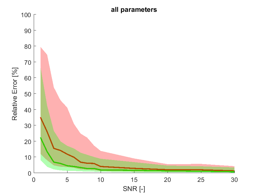
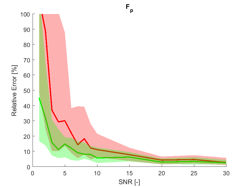
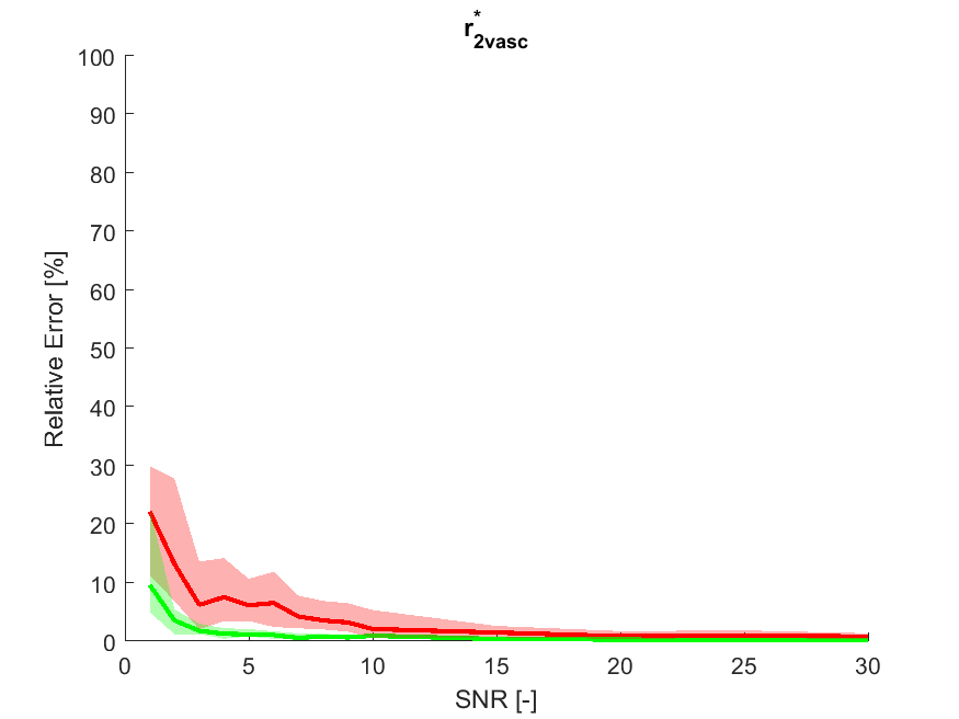
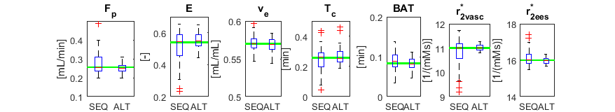
The estimation relative errors of the alternating optimization were significantly lower than for the sequential approach (Figure 1. and 2.), especially in the range of typical real-data SNR levels of 1-10. The most obvious improvement was in r2vasc* (Figure 3), r2ees* in almost the whole SNR range. The alternating approach boxplots of the prostate tumor parameters were systematically narrower and less biased in comparison with the sequential processing (Figure 4.). However, in case of glioblastoma, the algorithm provided worse results compared to sequential processing.Discussion
The presented alternating approach can provide a more robust perfusion parameter estimation than the sequential approach in the whole range of SNRs. The approach performs remarkably better in SNRs from 1 to 10, which is the usual noise level in real data. For higher SNR, the sequential processing is robust enough. With other optimization strategies, however more accurate results might be obtained. To solve problem with glioblastoma tissue, fitting errors of both approaches can be compared and the solution with lower error should be preffered. The alternating approach and the realism of the aaTH and GCM models will be validated on real data.Conclusion
The presented method can substantially improve the achievable precision of MRI quantitative perfusion analysis. The algorithm needs to be speeded up to make it feasible in clinical practice.Acknowledgements
The financial support of the Czech Science Foundation and the Ministry of Education, Youth and Sports of the Czech Republic (grants no. GA16-13830S and no. LO1212) is acknowledged.
References
1. Sourbron S, Heilmann M, Walczak C, Vautier J, Schad LR, Volk A. 2013. T2*-relaxivity contrast imaging: first results. Magn. Reson. Med. 69(5):1430–37.
2. Macícek O, Jirík R, Starcuk jr. Z. 2016. ESMRMB 2016, 33rd Annual Scientific Meeting, Vienna, AT, September 29 – October 1: Abstracts, Saturday. Magn. Reson. Mater. Physics, Biol. Med. 29(S1):247–400.
3. St Lawrence KS, Lee TY. 1998. An adiabatic approximation to the tissue homogeneity model for water exchange in the brain: I. Theoretical derivation. J. Cereb. Blood Flow Metab. 18(12):1365–77.
4. Koh TS. et al. 2001. The inclusion of capillary distribution in the adiabatic tissue homogeneity model of blood flow. Phys. Med. Biol. 46(5):1519–38.
5. Bartoš M, Keuen O, Jirík R, Bjerkvig R, Taxt T. 2010. Perfusion Analysis of Dynamic Contrast Enhanced Magnetic Resonance Images Using a Fully Continuous Tissue Homogeneity Model with Mean Transit Time Dispersion and Frequency Domain Estimation of the Signal Delay. Proc. Biosignal 2010 Anal. Biomed. Signals Images, pp. 269–74. Brno, Czech Republic: Brno University of Technology.
6. Coleman, T.F. and Y. Li. "An Interior, Trust Region Approach for Nonlinear Minimization Subject to Bounds." SIAM Journal on Optimization, Vol. 6, 1996, pp. 418–445.
7. Coleman, T.F. and Y. Li. "On the Convergence of Reflective Newton Methods for Large-Scale Nonlinear Minimization Subject to Bounds." Mathematical Programming, Vol. 67, Number 2, 1994, pp. 189–224.
8. Jirík R, Soucek K, Mézl M, Bartoš M, Dražanová E, et al. 2014. Blind deconvolution in dynamic contrast-enhanced MRI and ultrasound. Conf. Proc. Annu. Int. Conf. IEEE Eng. Med. Biol. Soc. IEEE Eng. Med. Biol. Soc. Annu. Conf. 2014:4276–79.
9. L. E. Kershaw and D. L. Buckley, “Precision in measurements of perfusion and microvascular permeability with T1-weighted dynamic contrast-enhanced MRI,” Magnetic Resonance in Medicine, vol. 56, no. 5, pp. 986–992, 2006.
10. Jacobs, G. J. Strijkers, H. M. Keizer, H. M. Janssen, K. Nicolay, and M. C. Schabel, “A novel approach to tracer-kinetic modeling for (macromolecular) dynamic contrast-enhanced MRI.” Magnetic Resonance in Medicine, vol. 75, no. 3, pp. 1142–1153, 2016.
11. M. C. Schabel, “A unified impulse response model for DCE-MRI,”Magnetic Resonance in Medicine, vol. 68, no. 5, pp. 1632–46, 2012.
12. Kratochvíla J, Jirík R, Bartoš M, Standara M, Starcuk jr. Z, Taxt T. 2016. Distributed capillary adiabatic tissue homogeneity model in parametric multichannel blind AIF estimation using DCEMRI. Magn. Reson. Med. 75(3):1355–65.
Figures