1882
Investigating the Sensitivity to Partial Volume Estimates of Partial Volume Correction for Single Postlabeling Delay Pseudo-continuous ASL1Institute of Biomedical Engineering, University of Oxford, Oxford, United Kingdom, 2Functional Imaging Unit, Department of Clinical Physiology, Nuclear Medicine and PET, Copenhagen University Hospital Rigshospitalet Glostrup, Copenhagen, Denmark, 3Department of Clinical Physiology, Nuclear Medicine and PET, Copenhagen University Hospital Rigshospitalet Blegdamsvej, Copenhagen, Denmark, 4St Hilda's College, University of Oxford, Oxford, United Kingdom
Synopsis
This work investigates the sensitivity of partial volume correction methods to partial volume estimates using single-PLD PCASL. Random and biased errors were applied to partial volume estimates to simulate the variabilities in tissue segmentation. The results have indicated that current partial volume correction methods trade off accuracy in spatial variations in CBF against sensitivity to noise and errors in the partial volume estimates.
Introduction
Single postlabeling delay (PLD) pseudo-continuous arterial spin labeling (PCASL) has been recommended as the standard implementation for cerebral perfusion quantification [1]. Due to the low spatial resolution of ASL data, precise perfusion quantification is limited by partial volume effects (PVE) [2]. Several partial volume correction (PVC) approaches have been developed including linear regression (LR) and the spatially regularized method [2, 3], but these have not yet been compared on the standard ASL acquisition. For both methods, it is critical to know the exact fraction of tissue in each voxel, the PV estimates. However, flaws in the segmentation process may introduce random and biased error in these PV estimates, which will affect the accuracy of PVC.
Here, we systematically investigate the sensitivity of PVC methods to variabilities in PV estimates. Random and biased errors were simulated, and the altered PV estimates are used in PVC on simulated Single-PLD PCASL data with a range of simulated gray matter (GM) CBF spatial variations. PVC methods were assessed by their ability to preserve spatial patterns and their sensitivity to errors.
Methods
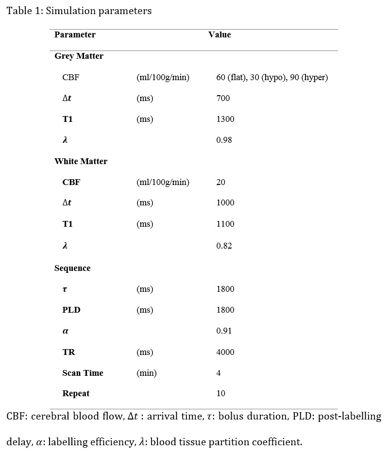
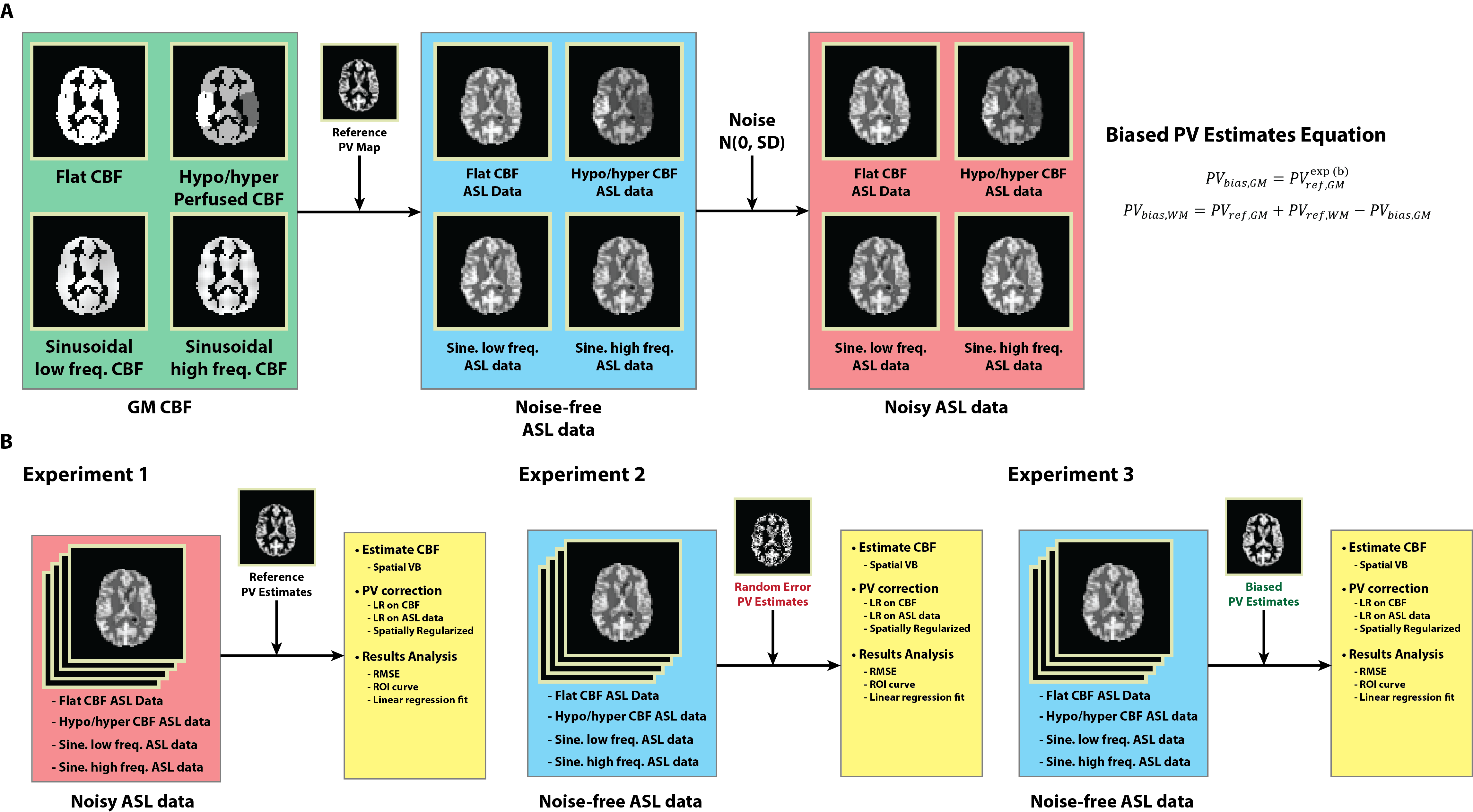
Four simulated PCASL ASL difference data were created by applying the general kinetic model as in [4] using the parameters listed in Table 1. GM CBF spatial variations were incorporated in the simulated data including flat GM CBF, slow and fast sinusoidal GM CBF variations, and hyper/hypo GM CBF to the left and right of the brain similar to [3]. White noise was added to the simulated data to represent MR background noise, and a total of 100 realizations for SNR=5, 10, 15, 20 were created. Figure 1A shows the simulation procedure.
The T1-weighted structural image of a healthy individual was registered to a calculated T1 image obtained by fitting a saturation recovery curve to ASL control data acquired in the same subject. The structural image was segmented, and PV estimates were transformed to ASL resolution. The resulting images were used as reference PV estimates. Random errors were drawn from a normal distribution N(0, SD) and added to the reference PV estimates to create random error PV estimates (equivalent to adding white noise), with SD=0, 0.05, ..., 0.2 and 100 realizations in each case. Biased PV estimates were produced by altering the reference PV estimates using a non-linear function in Figure 1. PVref and PVbias are the reference and biased tissue PV estimates respectively, 𝑏 is the bias factor with value of -0.5, -0.4, ..., 0.5. This function exchanges PV in GM for WM, assuming that there is some inherent bias in the PV estimation process between these two tissue types.
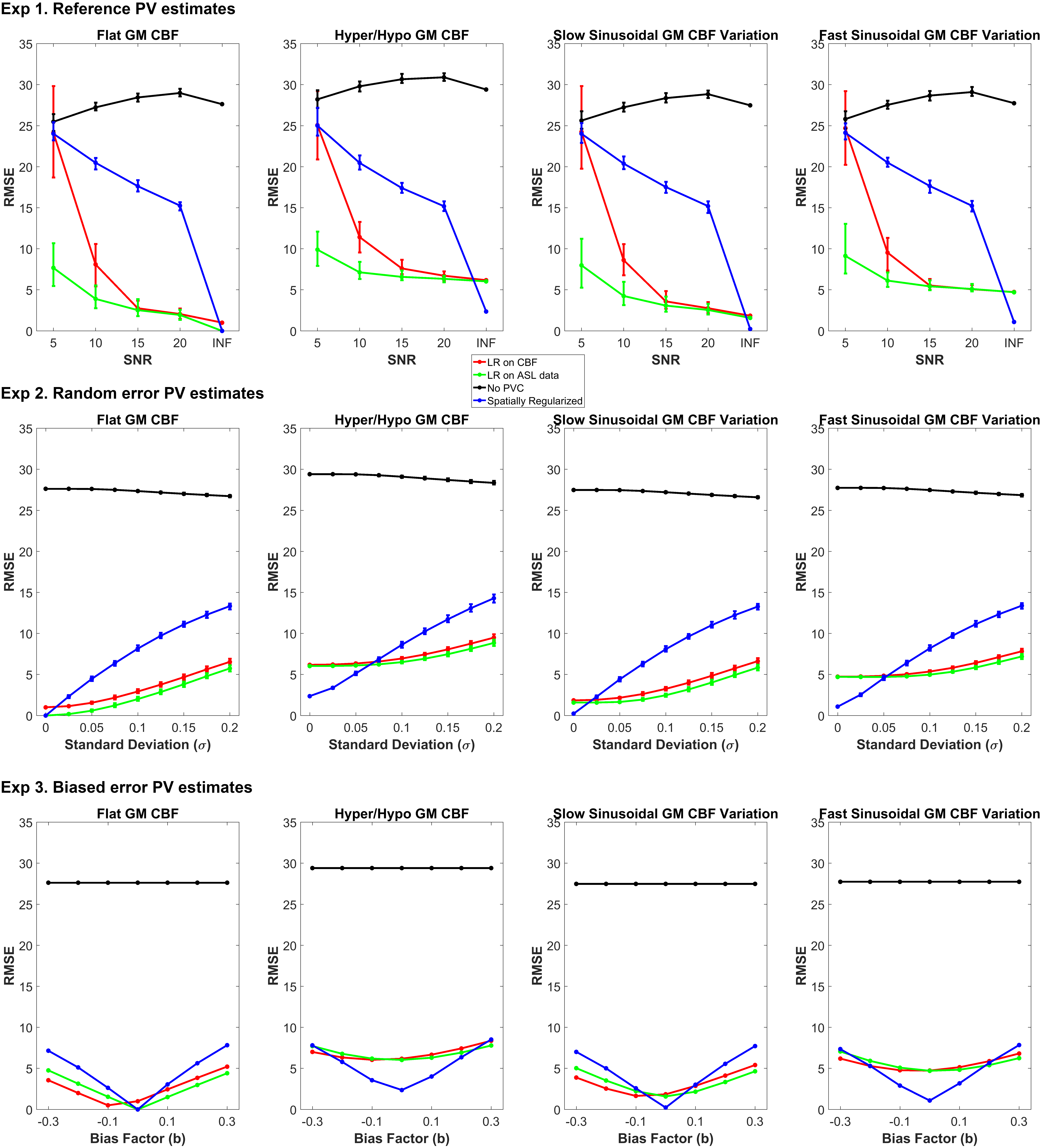
CBF was estimated by model-fitting using spatial Variational Bayesian method [5]. PVC was performed using three approaches: LR on CBF maps, LR on ASL data prior to CBF quantification, and the spatially regularized method where CBF is estimated at the same time as PVC. A kernel size of 5x5x1 was chosen for the two LR methods. Three experiments were conducted using different PV estimates, PVC using: (1) Reference PV estimates on noise-free and noisy data; (2) Random error PV estimates on noise-free data; (3) Biased error PV estimates on noise-free data. RMSE was computed between each estimated and simulated GM CBF. The ROI based analysis of [2] was extended for quantitative comparison of PVC performance by considering a linear regression of GM CBF and PVE in 10%- 90% range. The slope of the regression was compared on the basis that zero slope indicates GM CBF to be independent of GM PVE while positive and negative slope represents underestimation and overestimation at low ROIs respectively. Figure 1B shows the experimental design.
Results
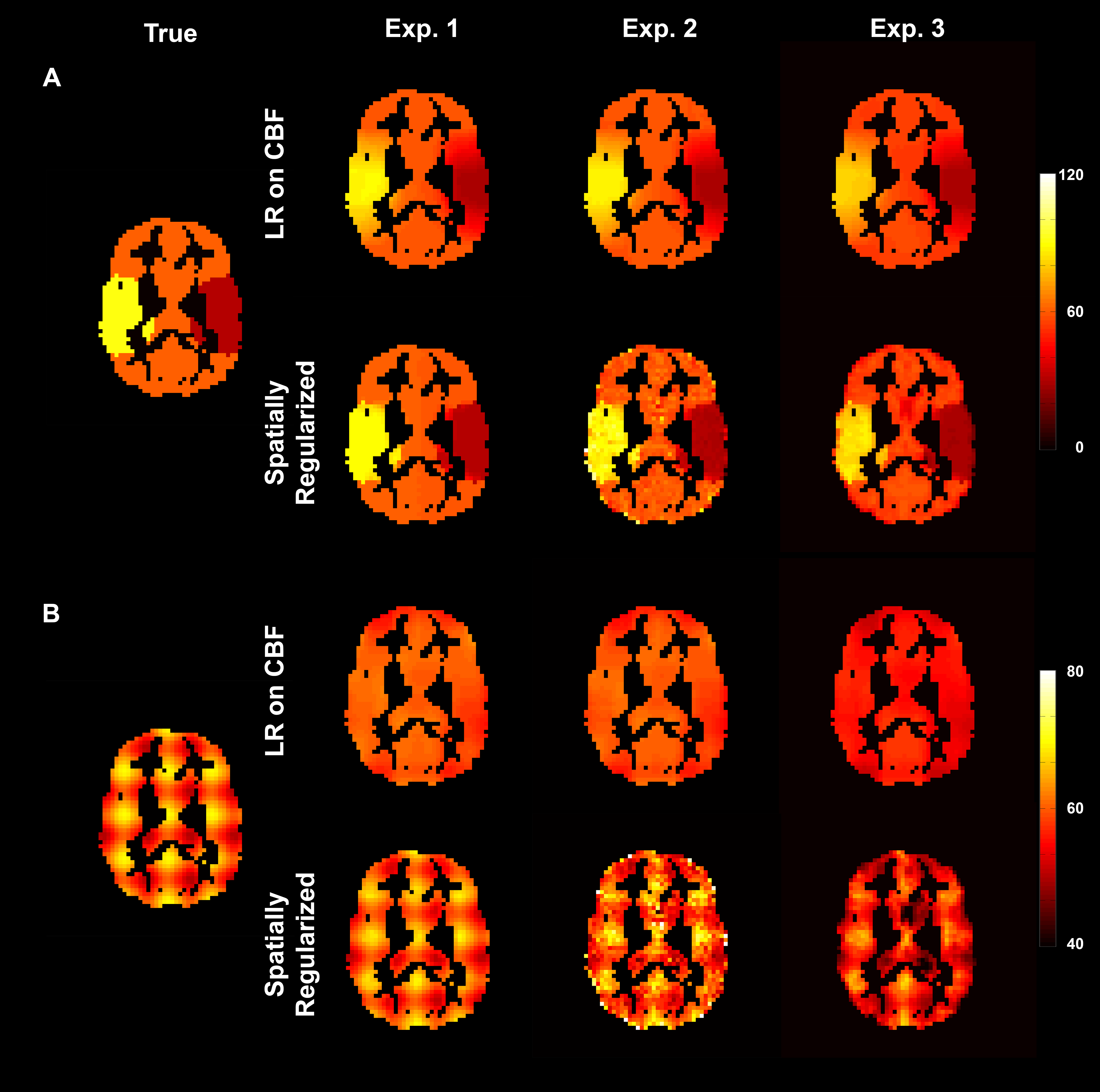
Figure 2 shows an example of estimated GM CBF maps. Figure 3 shows the RMSE between estimated and simulated GM CBF. Figure 4 shows the ROI analysis and estimated slope values for each experiment.Discussion
The findings of the study are: (1) all three PVC methods reduce the impact of PVE in CBF estimation substantially regardless of the variabilities in data and PV estimates; (2) the spatially regularized method was superior to the two LR methods in preserving spatial features but more sensitive to error in the PV estimates. PVE influence the GM CBF measures derived from ASL data when using the white paper recommendation. Although PVC can potentially correct for this, the existing methods trade off accuracy in spatial variations in CBF against sensitivity to noise and errors in the PV estimates. It is likely that similar conclusions would hold for other ASL acquisitions, and this is an area of ongoing investigation.Acknowledgements
The collaboration was facilitated by the COST Action BM1103 on “Arterial Spin Labeling Initiative in Dementia (AID)”.References
[1] D. C. Alsop, J. A. Detre, X. Golay, M. Günther, J. Hendrikse, L. Hernandez-Garcia, H. Lu, B. J. Macintosh, L. M. Parkes, M. Smits, M. J. P. van Osch, D. J. J. Wang, E. C. Wong, and G. Zaharchuk, “Recommended implementation of arterial spin-labeled perfusion MRI for clinical applications: A consensus of the ISMRM perfusion study group and the European consortium for ASL in dementia,” Magnetic Resonance in Medicine, 2014.[2] I. Asllani, A. Borogovac, and T. R. Brown, “Regression algorithm correcting for partial volume effects in arterial spin labeling MRI,” Magn. Reson. Med., vol. 60, pp. 1362–1371, 2008.[3] M. A. Chappell, A. R. Groves, B. J. MacIntosh, M. J. Donahue, P. Jezzard, and M. W. Woolrich, “Partial volume correction of multiple inversion time arterial spin labeling MRI data,” Magn. Reson. Med., vol. 65, pp. 1173–1183, 2011.[4] R. B. Buxton, L. R. Frank, E. C. Wong, B. Siewert, S. Warach, and R. R. Edelman, “A general kinetic model for quantitative perfusion imaging with arterial spin labeling.,” Magn. Reson. Med., vol. 40, pp. 383–396, 1998.[5] M. A. Chappell, A. R. Groves, B. Whitcher, and M. W. Woolrich, “Variational Bayesian Inference for a Nonlinear Forward Model,” IEEE Trans. Signal Process., vol. 57, no. 1, pp. 223–236, 2009.Figures