1849
Validating Particle Dynamics in Monte Carlo Diffusion Simulation using the Finite Element Method1Computer Science, Centro de Investigacion en Matematicas, Guanajuato, Mexico, 2Department of Computer Science and Centre for Medical Image Computing, University College London, London, United Kingdom
Synopsis
Monte-Carlo Diffusion Simulation (MCDS) is commonly used to develop and validate analytical models for quantifying tissue microstructure using diffusion MRI. However, the validation of the tools implementing MCDS has been limited, especially for complex domains, such as the extra-cellular space of brain tissue. To address this challenge, we propose a novel framework using the Finite Element Method (FEM), an established method for solving the diffusion equation with complex domains, to provide the ground-truth to assess MCDS. We demonstrate the framework by assessing how the accuracy of MCDS is influenced by the number of particles and the number of diffusion steps.
Purpose
Microstructure imaging with diffusion MRI is increasingly popular, enabling the estimation of specific white matter microstructure parameters, e.g. axon diameters and intra-cellular volume fractions1-3. The development and validation of these novel techniques have commonly relied on Monte Carlo Diffusion Simulation (MCDS) to provide the gold-standard for evaluation4-6. Given its importance, MCDS itself deserves careful validation. However such validation has been limited6-9, especially for simulation in complex domains, such as the extra-cellular space of brain tissue. This work provides a framework for systematically assessing particle dynamics in MCDS with arbitrary domains using the Finite Element Method (FEM). The experiments demonstrate the influence of MCDS user-parameters on the simulation accuracy.Methods
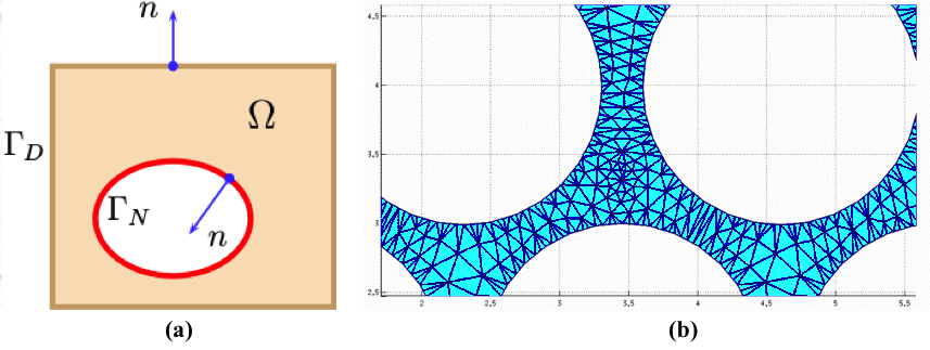
Framework Overview: The diffusion equation, which governs the diffusion process, is solved using a FEM based numerical solver of partial differential equation (PDE).10 This allows the particle density distribution over time to be computed accurately and robustly for arbitrary domains when the analytical solutions are unavailable. This ground-truth (GT) is used to quantitatively assess the particle density distribution determined from MCDS. GT Computation: The GT spatiotemporal particle density distribution $$$u=u(x,y,t)$$$ on an arbitrary domain Ω, Figure 1(a), is computed as follows. A mesh with elements $$$e$$$ is introduced in Ω, Figure 1(b). Second, to generate an easy-to-validate experiment, the density at time $$$t$$$=0 is concentrated at the elements associated to a single user-defined node with coordinates $$$(x_0,y_0)$$$ by using a Kronecker delta in the PDE initial condition $$$u_0(x,y) = \delta_{x_0,y_0}(x,y)$$$. Finally, FEM solves the diffusion equation $$$u_t=D(u_{xx}+u_{yy})$$$ for a given diffusion coefficient $$$D$$$.10 The solution provides element-wise densities $$$u_e$$$ computed as the average of the values at the vertices of element $$$e$$$ normalized by its area. MCDS Setting and Execution: The FEM mesh is also introduced in the MCDS domain to set up a rigorous correspondence between the MCDS starting configuration and the FEM initial condition $$$u_0(x,y)$$$. The MCDS particles are thus seeded according to a rejection-sampling strategy over the mesh elements connected to the node at $$$(x_0,y_0)$$$ to interpolate the initial density. By using this setting, the MCDS generates FEM-comparable element-wise spatiotemporal particle densities, $$$u^{MC}_e$$$, computed as the number of particles inside a FEM element $$$e$$$ divided by its area. Validation: The deviation of the MCDS simulation with respect to the FEM’s GT is measured by the sum of squared error in the particle density estimates over the set of mesh nodes $$$E$$$: $$\epsilon_u = \sum_e^E ( u^{MC}_e - u_e )^2,$$ where the final densities $$$u^{MC}_e$$$ and $$$u_e$$$ are normalised by taking into account all the element's values.
Experiments and Results
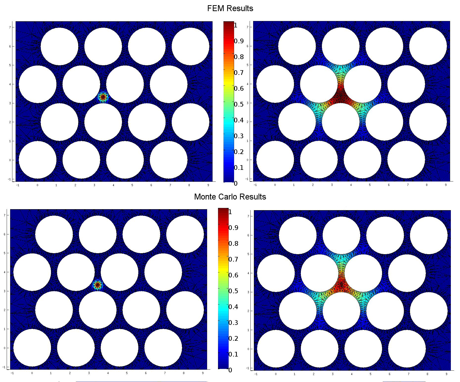
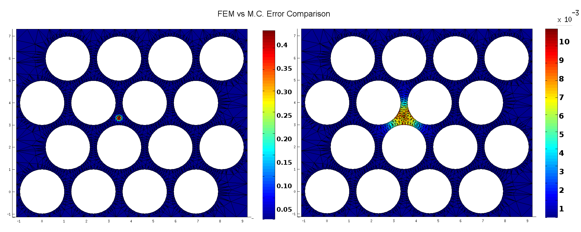
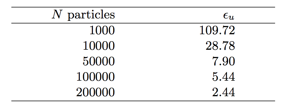
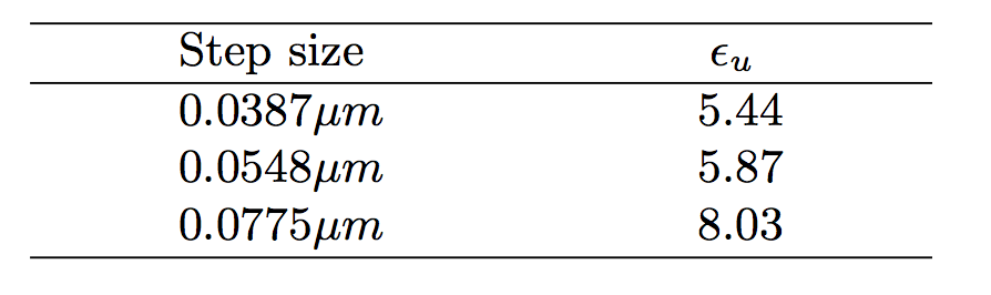
As a proof of concept, we illustrate the proposed framework by assessing the performance of an in-house tool for MCDS11 in a complex 2D domain that mimics the extracellular space of parallel axons. Experimental settings: We used a FEM mesh representing 2D circular walls (radius $$$R=1 \mu m$$$ and separation of $$$0.4 \mu m$$$) to study the extra-axonal particle dynamics, Figure-1(b). The experiments use $$$D=0.5 \frac{\mu m^2}{ms}$$$ and duration $$$dt=1 ms$$$, these values have been chosen to keep the FEM computation tractable. The initial experiments use $$$N=200000$$$ particles and $$$T = 1000$$$ steps for MCDS, and the corresponding $$$500$$$ time steps for FEM. Subsequently, we vary the MCDS parameters systematically to quantitatively measure the performance of the resulting simulations: a) we increase $$$N$$$ from $$$1000$$$ to $$$200000$$$, and b) the step size was increased from $$$0.0387\mu m$$$ to $$$0.0775\mu m$$$. Qualitative evaluation: A similar pattern of spreading particle densities is seen for the MCDS and the FEM solution, as illustrated by two different time points in Figure 2. These small differences in the density distributions are expected due to the discrete and stochastic nature of MCDS. Quantitative results: The $$$\epsilon_u$$$ map in Figure 3 is consistent with the qualitative evaluation on Figure 2, it shows a small and homogeneous error near the center. In next experiment, Table 1 shows how the changes in $$$N$$$ are reflected in the value of $$$\epsilon_u$$$. Finally, the impact associated with the change in $$$T$$$ is reported in Table 2. The results demonstrate the utility of the proposed framework for identifying the necessary settings for accurate MCDS.
Conclusions
We presented a framework to validate the correctness of MCDS stochastic outcomes on arbitrarily complex domains. The proposal was used to measure the impact on the simulations quality associated with the main MCDS variables, namely, number of particles, diffusion time, and time steps. The experiments demonstrate the framework is able to detect spurious deviations on the simulations.Acknowledgements
J. Rafael-Patiño was supported by a scholarship from CONACYT, Mexico. A. Ramirez-Manzanares was partially supported by SNI-CONACYT, Mexico, (Grant 169338) .References
1. Assaf Y., Blumenfeld-Katzir T., et al. Axcaliber: A method for measuring axon diameter distribution from diffusion MRI. Magnetic Resonance in Medicine. 2008; 59(6): 1347-1354.
2. Alexander D.C., Hubbard P.L., et al. Orientationally invariant indices of axon diameter and density from diffusion MRI. NeuroImage. 2010; 52(4): 1374-1389.
3. Zhang H., Schneider T., et al. NODDI: Practical in vivo neurite orientation dispersion and density imaging of the human brain. Neuroimage. 2012; 61(4): 1000-1016.
4. Stanisz J., Wright A., et al. An analytical model of restricted diffusion in bovine optic nerve. Mag. Res. in Med. 1997;37(1):103–111.
5. Yeh C-H., Tournier J.D., et al. The effect of finite diffusion gradient pulse duration on fibre orientation estimation in diffusion MRI. NeuroImage. 2010; 51(2):743-751.
6. Fieremans E., De-Deene Y., et al. Simulation and experimental verification of the diffusion in an anisotropic fiber phantom. J. of Mag. Reson. 2008; 190(2):189-99.
7. Hall M. G., Alexander D.C. Convergence and Parameter Choice for Monte-Carlo Simulations of Diffusion MRI. 2009; 28(9):1354-64.
8. Landman B.A., Farrell J.A, et al. Complex geometric models of diffusion and relaxation in healthy and damaged white matter. 2010;23(2):152-162.
9. Yeh C-H., Schmitt B., et al. Diffusion Microscopist Simulator: A General Monte Carlo Simulation System for Diffusion Magnetic Resonance Imaging. PLOS ONE. 2013; 8(10):e76626.
10. Quek S., Liu G.R.: The finite element method: A practical course, chap. FEM for heat transfer problems. Elsevier. 2003.
11. Jonathan Rafael-Patino. Design and Validation of a Robust Diffusion-Weighted-MRI Monte Carlo Simulator. Master Thesis at Centro de Investigation en Matematicas A. C. 2015; http://www.cimat.mx/es/Tesis_digitales .
Figures