1845
Benefits of flow, eddy current and concomitant field compensation in diffusion weighted MRI1Medical Physics in Radiology, German Cancer Research Center, Heidelberg, Germany, 2Joint Department of Physics, The Institute of Cancer Research and The Royal Marsden NHS Foundation Trust, London, United Kingdom, 3Institute of Radiology, University Hospital Erlangen
Synopsis
Diffusion-weighted MRI suffers from artifacts due to flow, concomitant fields and eddy currents. Different combinations of compensation for these effects were examined in phantom measurements as well as in vivo in the brain and in the prostate. The signal variations in the phantom measurements indicate that it could be advantageous to simultaneously compensate of all three effects over only flow and concomitant field compensation. This could not be seen in the in vivo results, where flow and concomitant field compensation proved to be as good as the full compensation.
Purpose
Flow-compensation can yield additional information in diffusion MRI1,2, but it can be prone to the same kind of artifacts as other diffusion sequences such as those originating from eddy currents3 or concomitant fields4. For this reason, a sequence was developed that allows the simultaneous compensation of flow, eddy currents and concomitant fields in order to assess, which of these compensations are of importance in flow-compensated diffusion weighted imaging.Methods
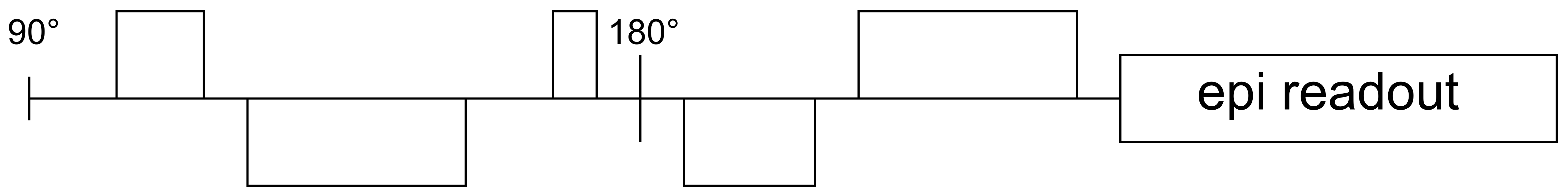
The scheme of the sequence, that was examined is shown in Fig. 1. Gradient durations and times between gradients were varied to find a solution minimizing the impact of the specified effect (flow, eddy current, concomitant field) or combinations of them, while maximizing the b-value. The timing parameters were allowed to be zero, which means that not all gradient pulses were used in all compensation schemes.
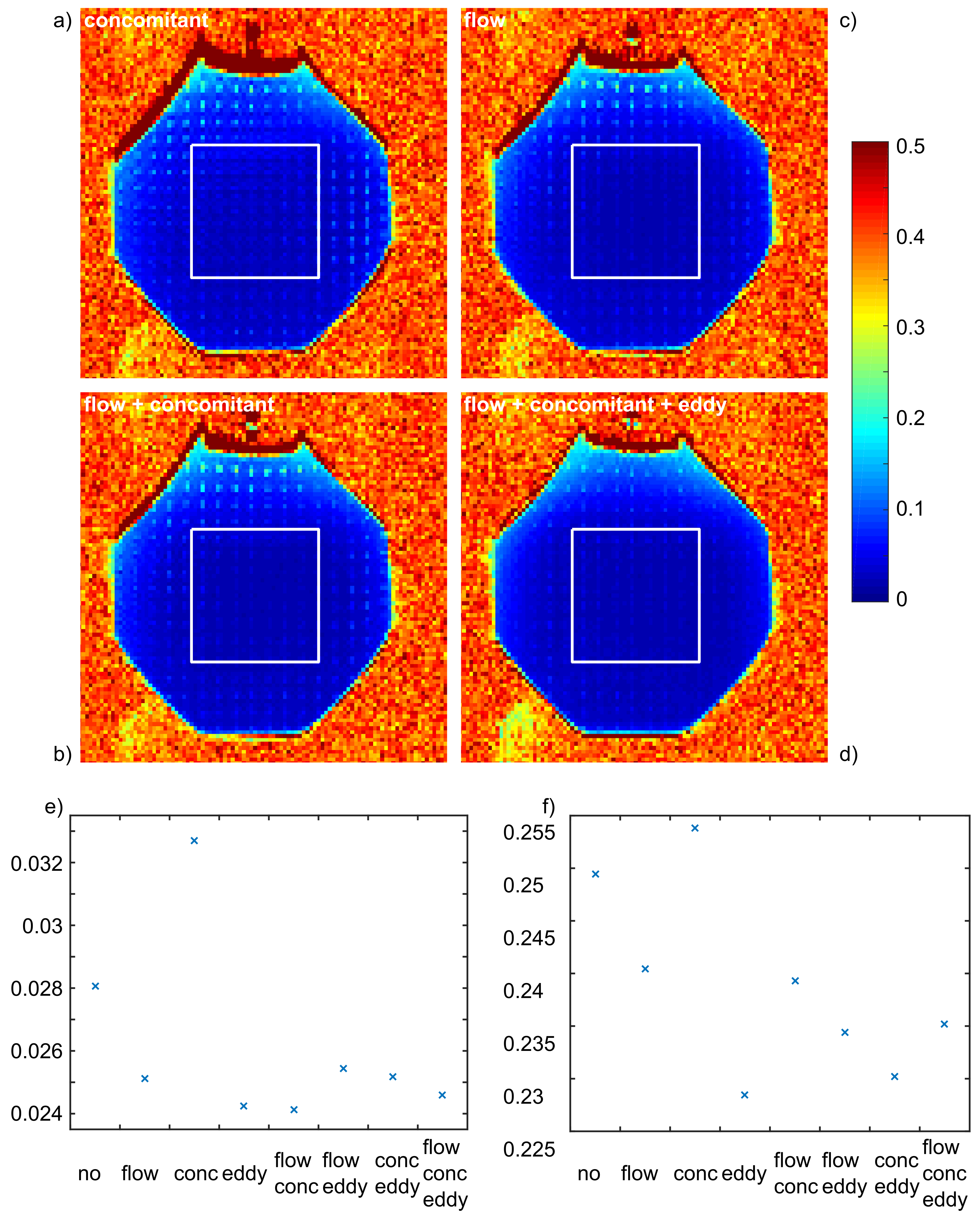
To verify the eddy current compensation, a phantom was used, which consists of plastic rods arranged on a regular grid that are immersed in water. This phantom was imaged with 64 different diffusion directions and a constant b-value of 1000 s/mm² and the coefficient of variation (CV) of the signal was calculated. Imaging parameters of the echo planar sequence were: TE/TR=90/4000 ms, FoV=450$$$\times$$$432 mm², nominal resolution=4.5$$$\times$$$4.5 mm², slice thickness=5 mm, 10 slices, pixel bandwith=2940 Hz and partial Fourier factor=6/8. The images were acquired with the build-in body coil.
To demonstrate the possible usefulness of the compensation,
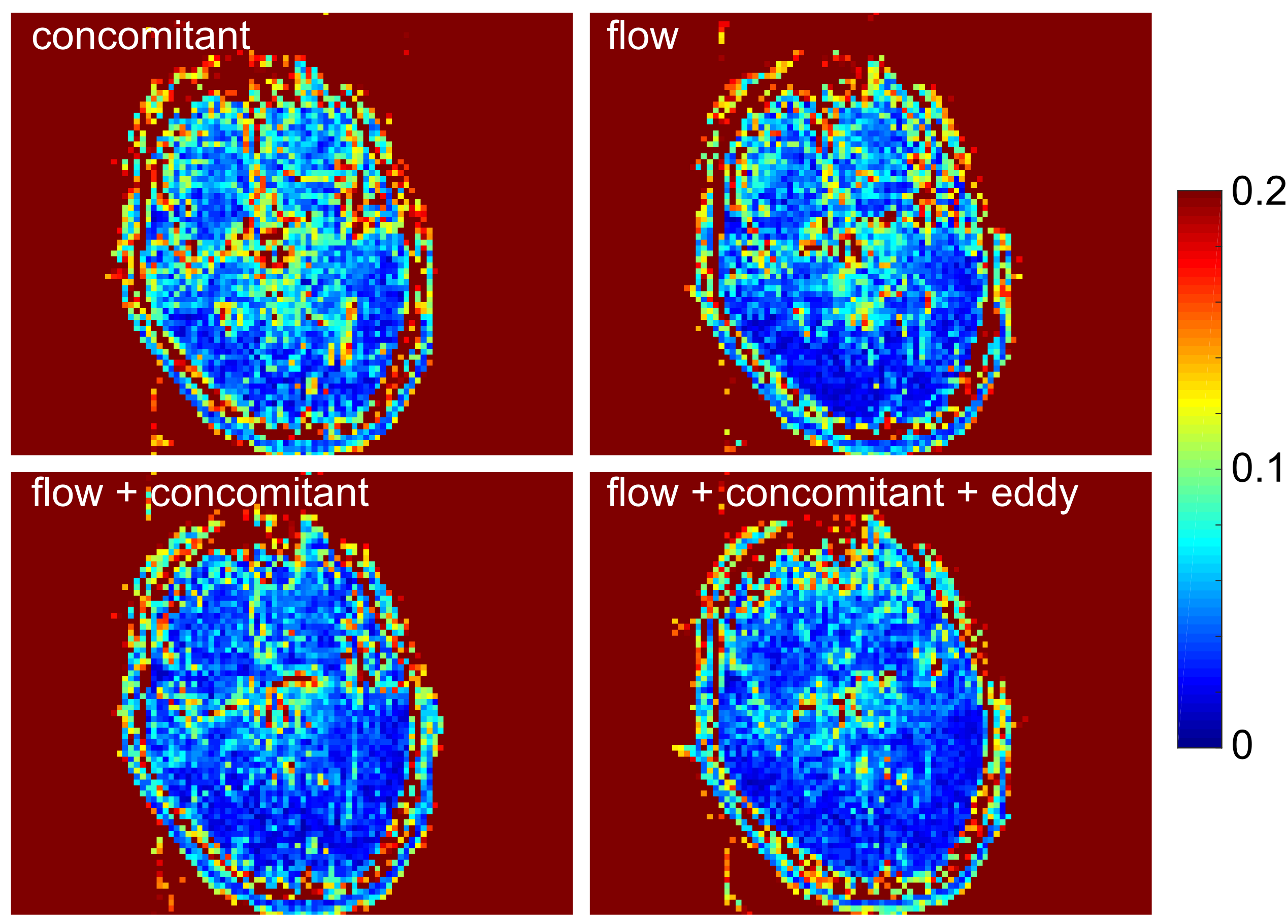
brain imaging of a healthy volunteer was performed. Ten repetitions of a diffusion
tensor imaging scheme with three b-values (0, 500, 1000 s/mm²) and six diffusion
directions were performed. For each repetition, a tensor fit was performed on a
voxel by voxel basis and the mean diffusivity MD was calculated. Then, the CV
of the MD over the 10 repetitions was determined. Other parameters of the echo
planar sequence were: TE/TR=75/5500 ms, FoV=218$$$\times$$$280 mm², nominal
resolution=2.8$$$\times$$$2.8 mm², slice thickness=5 mm, pixel bandwith=2940 Hz,
Grappa factor=2 and partial Fourier factor=6/8.
The images were acquired using a 64 channel head coil.
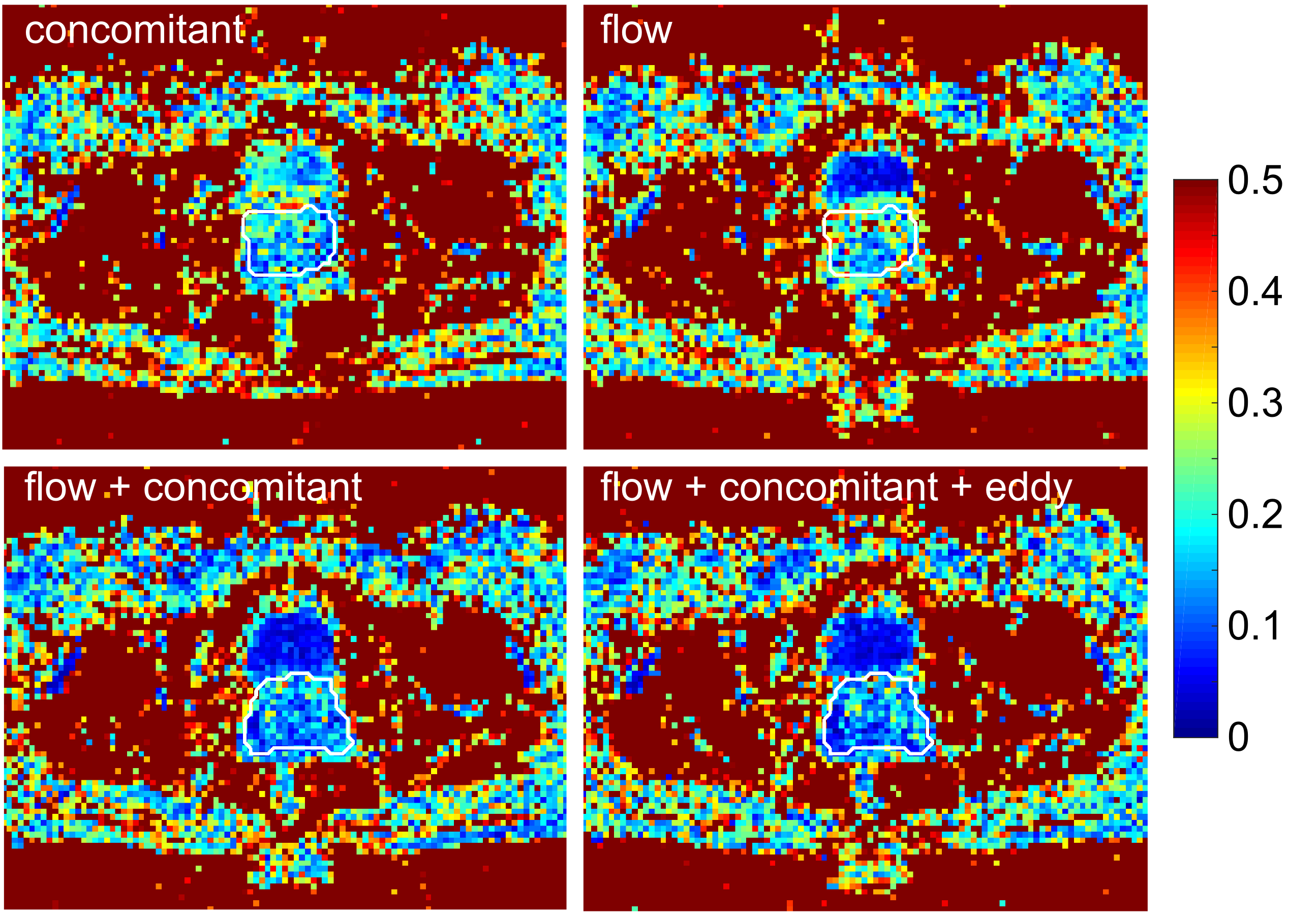
Additionally, prostate images of one volunteer were acquired. Five repetitions and three directions were used, with the b-values of 0, 250, 500, 1000 s/mm². For each repetition, the MD was calculated using the trace-weighted images and then the CV of the MD was determined. The other sequence parameters were: TE/TR=85/3300 ms, FoV=280$$$\times$$$218 mm², nominal resolution=2.8$$$\times$$$2.8 mm², slice thickness 5 mm, 10 slices, pixel bandwith=2780, Grappa factor=2 and partial Fourier factor=6/8. The images were acquired using a 18 channel flex coil.
All measurements were performed at a 3T scanner (Magnetom
Prismafit, Siemens Healthcare, Erlangen) and the maximal gradient amplitude was
limited to 75 mT/m.
Results
In Fig.2a)-d), the CV maps of the phantom are shown for different compensation combinations, while Fig.2e) shows the mean CV inside the ROI depicted in the maps and Fig.2f) shows the mean CV over the whole image. Figures 3 and 4 show the in vivo CV maps for the brain (Fig.3) and the prostate (Fig.4) in an exemplary slice. All maps show only the compensation combinations concomitant field, flow, concomitant field & flow, and all three.
In the brain measurements, the CV reduces when using a flow-compensation.There are only minor improvements visible when adding eddy current compensation.
The prostate images show the main improvement by adding concomitant field and flow compensation, while eddy current compensation doesn’t improve the stability further.
Discussion
The measurements of the grid phantom can be regarded as a way to determine the effectiveness of the eddy current compensation. The mean CV inside the chosen ROI shows only minor differences in the compensation schemes, except for no or only concomitant field compensation. This is different if the whole phantom is considered. This can be understood by looking at the CV maps, where the signal variations get higher the further it is away from the isocenter.
The variations in the MD measurements in the brain are partly due to pulsation, which explains the improvement by using flow compensation.
The flow-compensation used here is partly eddy current compensated. Depending on the actual timing, the use of an additional concomitant field compensation can lead to a better eddy current compensation. This seems to be the case in the in vivo measurements.
Conclusion
Diffusion measurements in flow-compensated MRI get more stable using additional concomitant field compensation. Additionally using eddy current compensation yielded little to no benefit in the current evaluation and can be neglected so that higher b-values can be used in the same TE.Acknowledgements
Financial support by the DFG (grant no. KU 3362/1-1 and LA 2804/2-1) is gratefully acknowledged.References
1. Ahlgren A, Knutsson L, Wirestam R, Nilsson M, Stahlberg F, Topgaard D, Lasic S. Quantification of microcirculatory parameters by joint analysis of flow-compensated and non-flow-compensated intravoxel incoherent motion (IVIM) data. Nmr in Biomedicine 2016;29(5):640-649.
2. Wetscherek A, Stieltjes B, Laun FB. Flow-compensated intravoxel incoherent motion diffusion imaging. Magnetic Resonance in Medicine 2015;74(2):410-419.
3. Mueller L, Wetscherek A, Kuder TA, Laun FB. Eddy current compensated double diffusion encoded (DDE) MRI. Magnetic Resonance in Medicine 2015:n/a-n/a.
4. Baron CA, Lebel RM, Wilman AH, Beaulieu C. The effect of concomitant gradient fields on diffusion tensor imaging. Magn Reson Med 2012;68(4):1190-201.
Figures