Synopsis

We discuss the usage of a recently-proposed diffusion-sensitising gradient waveform for the purpose of imaging the potential energy landscape in which water molecules diffuse. The energy landscape encodes information about bulk heterogeneities of the medium as well as effects such as adsorption at the boundaries.

Introduction

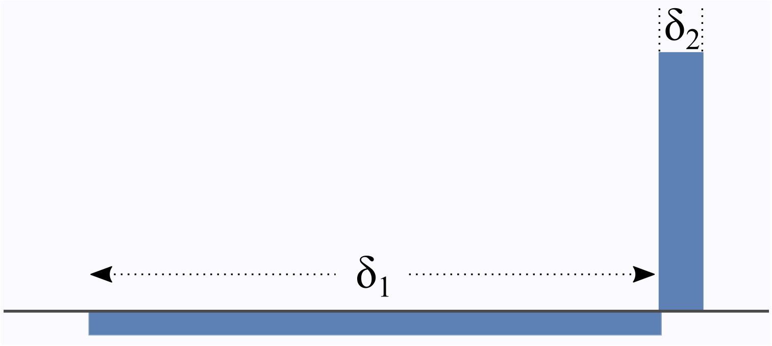
The mesoscopic structure of porous media and biological tissue can be probed by NMR experiments sensitised to diffusion of water through the usage of appropriate magnetic field gradients. Recently, the gradient waveform illustrated in Figure 1 was shown to allow the Fourier transform of the pore space to be measured [1,2], as opposed to typically-employed gradient sequences that yield only its power spectrum. Here, we argue that this sequence can measure another quantity that can be more relevant than the pore space function in various situations.

A useful point of view for diffusion in complex media is to consider the process under the influence of a potential energy landscape. This can take into account inhomogeneities in the bulk, as well as represent boundaries if needed, in a more wieldy manner mathematically. The latter is, for instance, the case for diffusing particles that experience partial adhesion to boundaries; such processes are hypothesized to make diffusion-weighted MRI signal sensitive to neuronal activation [3].

Theory

The diffusion-weighted NMR signal is the expectation value,

$$ S = \left< e^{-i \gamma \int_0^t {\rm d} s \, \boldsymbol G (s) \cdot \boldsymbol x(s)} \right> \ , $$

of the complex phase accumulated by the spin-carriers. We apply Laun's gradient sequence [1,2] shown in Figure 1 featuring a long pulse followed by a short pulse,

$$ \boldsymbol G(s) = \left\{ \begin{array}{lll} -\boldsymbol G &,& 0<s<\delta_1 \ , \\ \tfrac{\delta_1}{\delta_2} \boldsymbol G &,& \delta_1<s<\delta_1+\delta_2 =t \ . \end{array} \right. $$

When the wavevector $$$\boldsymbol q$$$ is defined as $$$\boldsymbol q= \gamma \delta_1 \boldsymbol G$$$, we obtain

$$ S = \left< e^{i \boldsymbol q \cdot \!\left[ \frac1{\delta_1} \int_0^{\delta_1} {\rm d} s \, \boldsymbol{x}(s)\right]} e^{-i \boldsymbol{q} \cdot \!\left[ \frac1{\delta_2} \int_{\delta_1}^t {\rm d} s \, \boldsymbol{x}(s) \right]} \right> \ . $$

The two exponents can be envisioned as the centers of mass of the random trajectories in their respective integration intervals [4]. We will consider the long-time sharp-pulse limit, $$$t \to \infty$$$ and $$$\delta_2/\delta_1 \to 0$$$. The long-time limit of the time average $$$(1/\delta_1) \int_0^{\delta_1} {\rm d} s \, \boldsymbol{x}(s)$$$ must be equal to the statistical average $$$\left< \boldsymbol{x} \right>$$$, which is independent of time and trajectory. Therefore, the first phase factor drops out of the expectation value, and the signal becomes

$$ S (\boldsymbol{q}) = e^{i \boldsymbol{q} \cdot \left< \boldsymbol{x} \right>} \left< e^{-i \boldsymbol{q} \cdot \boldsymbol{x}(t) } \right> \ , $$

where the simplification of the second phase factor is due to its integration interval shrinking to a moment.

The distinction between this expression and Laun's is found in the underlying diffusion process being subject to a potential $$$V (\boldsymbol{x})$$$ rather than the restriction of pore space boundaries. In this case, $$$\left< \boldsymbol{x} \right>$$$ is not the center of mass of the pore space; instead it is the average position in the underlying potential landscape. Similarly, the expectation value of the phase is that determined by the asymptotic ($$$t \to \infty$$$) probability distribution $$$\rho (\boldsymbol{x}) \sim e^{-\beta V(\boldsymbol{x})}$$$ , where $$$\beta$$$ is the inverse thermal energy. Therefore, the dMRI signal yields the Fourier transform of the stationary distribution for the underlying potential landscape, with its mean shifted to the origin:

$$ S (\boldsymbol{q}) = \int {\rm d} \boldsymbol{x} \, \rho (\boldsymbol{x}) e^{-i \boldsymbol{q} \cdot \left( \boldsymbol{x} - \left< \boldsymbol x \right> \right) } \ . $$

Results and Discussion

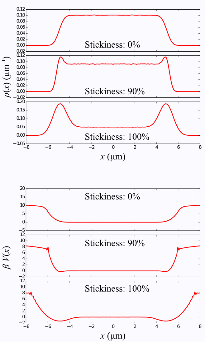
As an illustration, we have performed random walk simulations in a 1D box as well as simple monomial potential wells. For the box, the boundary conditions were either perfectly reflective, or sticky. In the latter case , after a random walker reaches the boundary, it has a certain probability of stepping away or remaining stuck until the next time step.

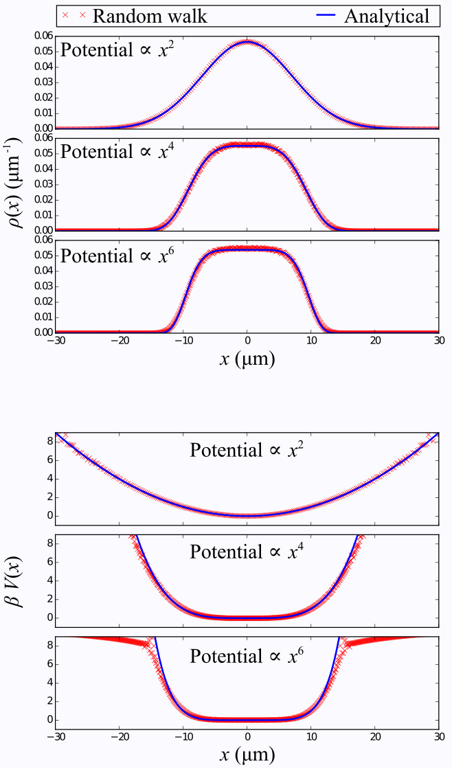
Figure 2 depicts distributions and corresponding potentials for the 1D box, obtained by measuring the signal followed by an inverse Fourier transform, as described previously. The adhesion effect is clearly seen as dips near the box boundaries. Random walk simulations performed in simple monomial potential wells demonstrate the recovery of the underlying analytic function, in Figure 3.

As shown in [5] for the case of anisotropic diffusion, treating disturbances to diffusion as variations in a potential landscape is a viable alternative in modeling diffusion in complex media. In this work, we have extended this approach to directly map the effective energy landscape that could influence the movements of water molecules.

Acknowledgements

References

[1] Laun et al., Phys Rev Lett, 107, 048102, 2011.

[2] Laun et al., Phys Rev E, 86, 021906, 2012.

[3] LeBihan, Phys Med Biol, 52, R57-R90, 2007.

[4] Mitra and Halperin, J Magn Reson A, 113, 94-101, 1995.

[5] Yolcu et al., Phys Rev E, 93, 052602, 2016.