Synopsis

We propose a Bayesian approach for improving the accuracy of diffusional kurtosis imaging in a small number of data acquisitions. Gaussian-approximated prior distributions are made from primary maximum-likelihood estimation (MLE). The approach was tested using a healthy volunteer data in which a part of signals was replaced with simulated glioma signals. Although the approach does not yield further improvement when MLE has a certain degree of accuracy, the approach has effect to reduce large misestimations and did not cause false shrinkage of dispersions that the sample parameters inherently have. The approach reduces the burden of data acquisition.

Purpose

Methods

Diffusional Kurtosis Imaging (DKI) Algorithms

Normalized signal of q-space imaging is expressed as $$$S(\vec{q})/S(0)=\int_{-\infty}^{\infty}P(\vec{R})\exp{(i\vec{q}\cdot\vec{R})}d^3R=1-q_iq_jM_{ij}/2+q_iq_jq_kq_lM_{ijkl}/4!+\cdots$$$, where $$$M_{ij}=\int_{-\infty}^{\infty}P(\vec{R})R_iR_jd^3R$$$, $$$M_{ijkl}=\int_{-\infty}^{\infty}P(\vec{R})R_iR_jR_kR_ld^3R$$$, and $$$\sum_i a_ib_i$$$ is written as $$$a_ib_i$$$. This is the characteristic function of the probability density function $$$P(\vec{R})$$$ for diffusion displacement $$$\vec{R}$$$. Using $$$b$$$ value,

$$\frac{S(b,\vec{n})}{S(0)}=1-bn_in_jD_{ij}+\frac{1}{6}b^2n_in_jn_kn_lD_{ijkl}+\cdots\hspace{1.7cm}(1),$$

where $$$D_{ij}=M_{ij}/(2t_d)$$$ and $$$D_{ijkl}=M_{ijkl}/(2t_d)^2$$$ with $$$t_d=\Delta-\delta/3$$$, and $$$\delta$$$/$$$\Delta$$$ are the duration/separation of motion probing gradient (MPG). The logarithm of the characteristic function is the cumulant generating function:

$$\log{\left\{\frac{S(b,\vec{n})}{S(0)}\right\}}=-bn_in_jD_{ij}+\frac{1}{6}b^2n_in_jn_kn_lV_{ijkl}+\cdots\hspace{1cm}(2),$$

where

$$V_{ijkl}=D_{ijkl}-D_{ij}D_{kl}-D_{jk}D_{li}-D_{kl}D_{ij}.$$

The kurtosis along a direction $$$\vec{n}$$$ is $$$K(\vec{n})=n_in_jn_kn_lV_{ijkl}/(n_in_jD_{ij})^2$$$.

We used two kinds of DKI algorithms: the characteristic function method (CFM)² and the cumulant generating function method (CGFM). The CFM uses Eq. (1) for fitting, and the CGFM, Eq. (2)³. We truncated the series of Eqs. (1) and (2) after the second-order terms. Kurtosis maps were made for mean, axial and radial kurtosis (K) defined in Ref. 4. To address systematic errors contained in DKI parameters we implement certain calibration procedures.

Bayesian Estimation

The likelihood function is

$$p(\vec{B}|\vec{X})\propto\exp{\left\{-\frac{1}{2}(A\vec{X}-\vec{B})^T\Sigma^{-1}(A\vec{X}-\vec{B})\right\}},$$

where $$$\vec{X}$$$ consists of $$$D_{ij}$$$'s and $$$V_{ijkl}$$$'s, $$$\vec{B}$$$ is composed of measured signals for given MPG directions ($$$\vec{n_i}$$$) and b-values ($$$b_i$$$), $$$A$$$ is a matrix composed of the $$$n_{ij}$$$'s and $$$b_i$$$'s, and $$$\Sigma^{-1}$$$ is a diagonal matrix. First, we estimate $$$D_{ij}$$$'s and $$$V_{ijkl}$$$'s by the maximum-likelihood estimation (MLE) using $$$p(\vec{B}|\vec{X})$$$:

$$\vec{X}_0=(A^T\Sigma^{-1} A)^{-1}A^T\Sigma^{-1}\vec{B}.$$

In this step, $$$\Sigma^{-1}$$$ was determined by the propagation law of error. We made a distribution for $$$\vec{X_0}$$$ in a slice by conducting the MLE for each voxel, and read off the median, $$$\langle\vec{X_0}\rangle$$$ and normalized interquartile ranges, $$$\Sigma_p^{1/2}$$$ of the distribution. We then made Gaussian prior distribution:

$$p(\vec{X})\propto \exp{\left\{-\frac{1}{2}(\vec{X}-\langle\vec{X_0}\rangle)^T\Sigma_p^{-1}(\vec{X}-\langle\vec{X_0}\rangle)\right\}}. $$

The Bayesian estimation was implemented using the posterior distribution:

$$p(\vec{X}|\vec{B})\propto p(\vec{B}|\vec{X})p(\vec{X}).$$

Estimates of $$$\vec{X}$$$ are expectation values:

$$\vec{X}_{\rm estimate}=(A^T\Sigma^{-1} A+\Sigma_p^{-1})^{-1}(A^T\Sigma^{-1}\vec{B}-\Sigma_p^{-1}\langle\vec{X_0}\rangle).$$

To calculate $$$\vec{X}_{\rm estimate}$$$, overall factor of $$$\Sigma^{-1}$$$ is necessary. We estimated it from the residuals obtained in MLE at the first step.

Data Acquisition and Simulated Glioma Signals

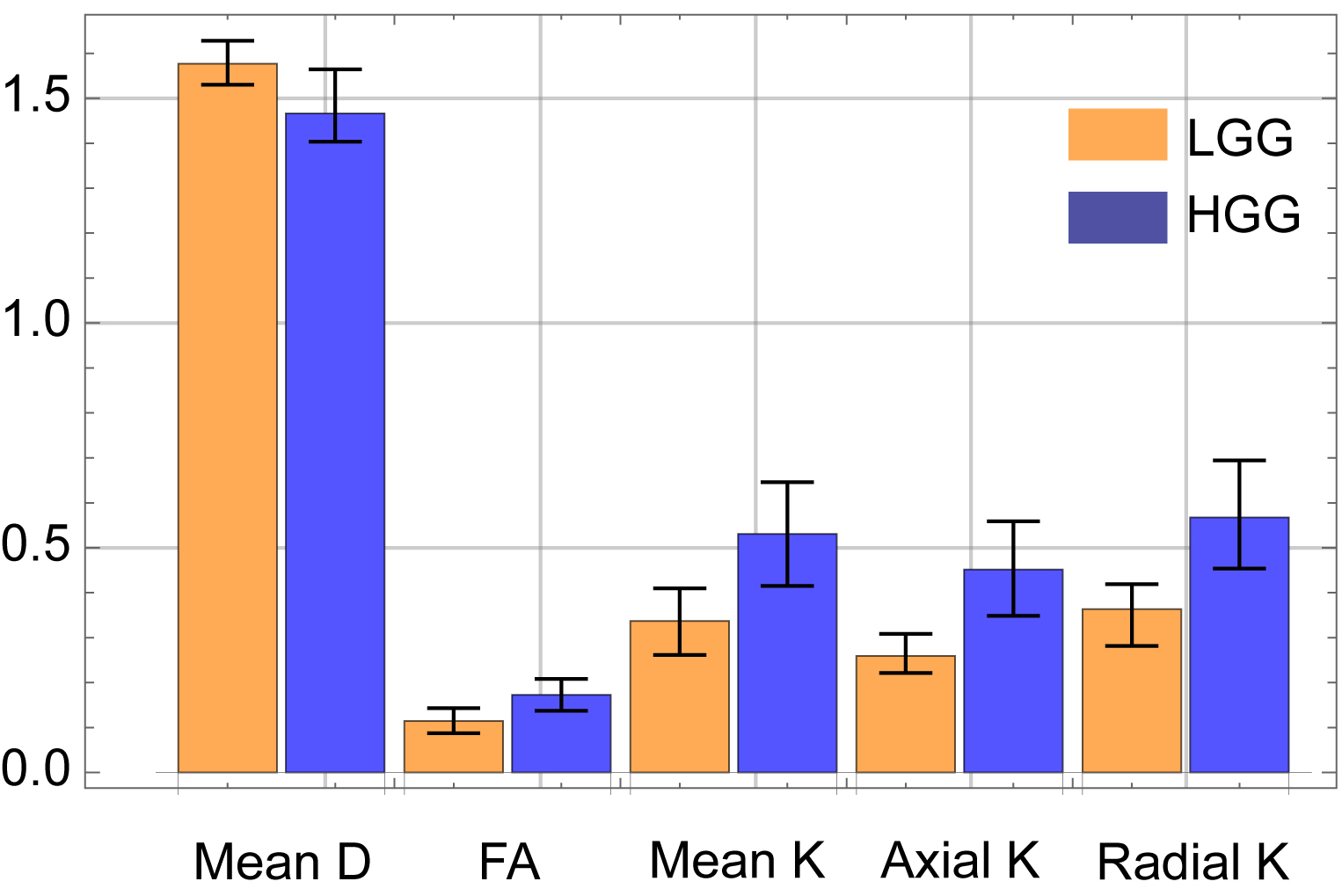
A healthy male volunteer was scanned on 3T Philips Ingenia system with TE/TR=128/12864 ms, NSA=1, isotropic voxel of 2×2×2 mm³. DWIs were acquired along 32 gradient directions with b=0,200,400,1000,1500,2000,2500 s/mm². The data were thinned out as appropriate to test our approach. We made simulated DWI signals for gliomas using the bi-exponential (exp.) model and replaced a part of acquired signals with them. For the model parameters we referred Refs. 5 and 1, and made 20 signals for high and low grade gliomas by fluctuating the parameters. True values of the DKI parameters for the sample are shown in Fig. 3.

Results

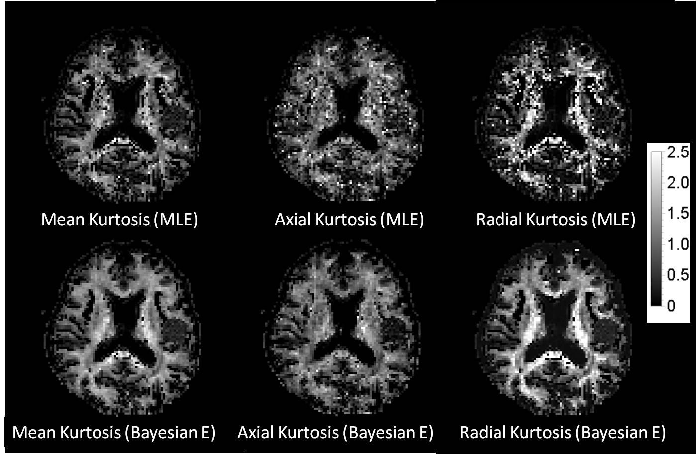
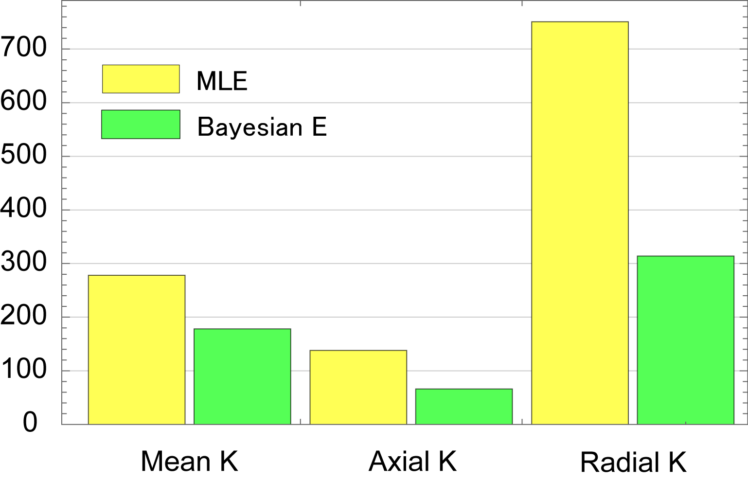
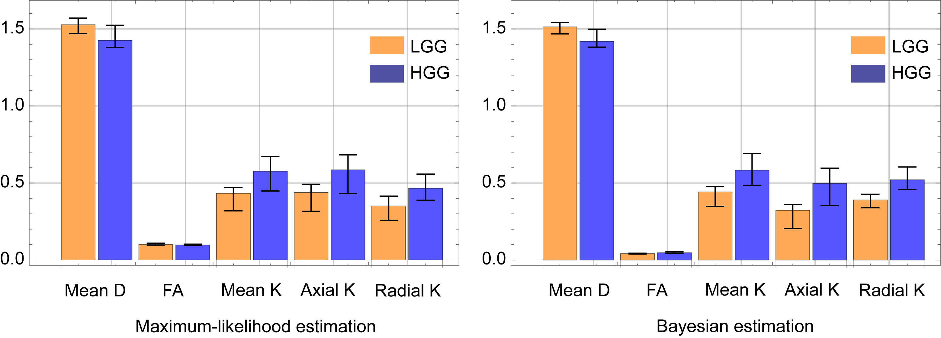
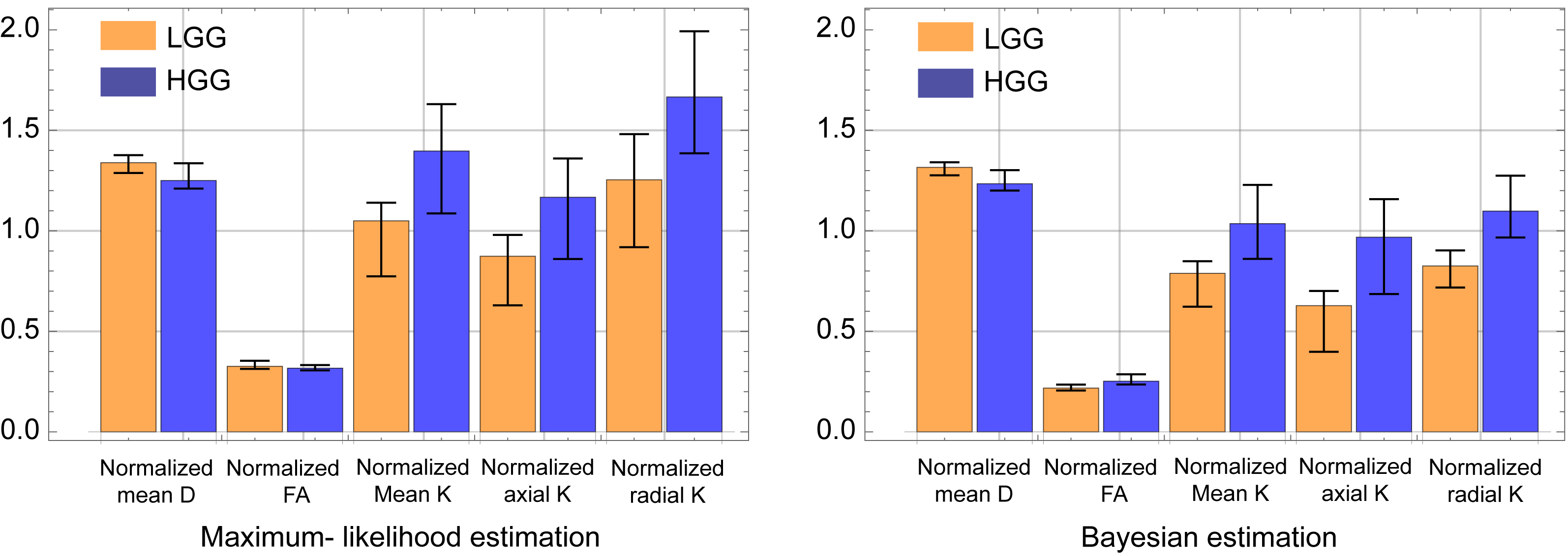
We only show the results obtained by CGFM for b=0, 1000, 2500 s/mm² and 16 gradient directions in this abstract. Kurtosis map and the numbers of the outlier-voxels were shown in Figs. 1 and 2, respectively. Imaging qualities were clearly improved by the Bayesian estimation. Medians and interquartile ranges of estimated parameters for the simulated glioma samples are shown in Fig. 4, and the normalized values to the contralateral normal-appearing white matter are shown in Fig. 5. All medians in Figs. 4 and 5 were significantly different between low and high grades (P<0.05). Overlaps of interquartile ranges between low and high grade gliomas tend to reduce in the Bayesian estimation, and especially for normalized parameters, error bars become smaller than those of MLE. The results not shown in this abstract indicated similar trends. In particular, the poorer the results of MLE are, the more Bayesian estimations become effective.

Discussion

The Bayesian approach has effect to reduce large misestimation and does not cause false shrinkage of dispersions that the sample parameters inherently have⁶. The approach is, however, less able to reduce small estimation error, and thus when MLE has a certain degree of accuracy, the approach does not yield further improvement. The phenomena are attributed to the Gaussian assumption for the prior distributions. If the actual distribution has multi-peak, the Gaussian-approximated distribution becomes broad as contains the peaks inside. The fact explains the above mentioned phenomena. Further improvement may be possible by a more rigorous treatment for the prior distribution with trading off the merit of simplification of the calculation due to the Gaussian approximation.

Conclusions

Acknowledgements

References

1. Van Cauter, Veraart J, Sijbers J, et al. Gliomas: diffusion kurtosis MR imaging in grading. Radiology 2012;263(2):492-501.

2. Umezawa E, Yoshikawa M, Yamaguchi K, et al. q-Space imaging using small magnetic field gradient. Magn Reson Med Sci. 2006;5(4):179-189.

3. Jensen JH, Helpern JA, Ramani A, et al. Diffusional kurtosis imaging: the quantification of non-gaussian water diffusion by means of magnetic resonance imaging. Magn Reson Med. 2005;53(6):1432-1440.

4. Tabesh A, Jensen JH, Ardekani BA, et al. Estimation of tensors and tensor-derived measures in diffusional kurtosis imaging. Magn Reson Med. 2011;65(3):823-836.

5. Maier SE, Sun Y, Mulkern RV. Diffusion imaging of brain tumors. NMR Biomed. 2010;23(7):849-864.

6. Orton MR, Collins DJ, Koh DM. Improved intravoxel incoherent motion analysis of diffusion weighted imaging by data driven Bayesian modeling. Magn Reson Med. 2014;71(1):411-420.