1767

Fast Linear Fitting of Bi-Exponential Intra-Voxel Incoherent Motion (IVIM) Models

Eric Thomas Peterson¹, Natalie May Zahr^2,3, Edith Vioni Sullivan², and Adolf Pfefferbaum¹

¹Biosciences, SRI International, Menlo Park, CA, United States, ²Psychiatry and Behavioral Sciences, Stanford University, Stanford, CA, United States, ³Bioscience, SRI International, Menlo Park, CA, United States

Synopsis

This work introduces an extremely fast (whole image in ~5s) IVIM fitting procedure based on two sequential linear fits and demonstrates that it is comparable to the more traditional but much slower non-linear fitting. This method is valuable because current fitting methods typically take a significant amount of time, typically from minutes to hours, due to their iterative and non-linear nature. Therefore, this technique can be used as a fitting method alone and also as a way to seed more advanced techniques with accurate starting values.

Purpose

Intra-voxel incoherent motion (IVIM) can probe both diffusion and flow by using a range of b-values, typically 0 to <1000 (s/mm²)^1–3. Lower b-values are primarily sensitive to capillary-level flow, and higher b-values are sensitive to tissue diffusion. This ability to measure both diffusion and flow in a single scan is desirable for studies where both metrics are needed, such as in evaluating the effects on the brain of alcoholism^4,5 or stroke³. Normally, IVIM data are fitted in multiple stages^1,2 and common approaches use nonlinear fitting^1,3,6,7. However, these approaches are often too slow to be of clinical use, taking from minutes to hours. This work introduces a fast IVIM fitting procedure (whole 3D image in ~5s) based on two sequential linear fits and demonstrates that it is comparable to the more traditional non-linear fitting.

Theory

Equation 1 shows the IVIM signal equation assuming flow (fe^-bD*) and diffusion ((1-f)e^-bD) compartments. The fitted parameters are S0 (signal), f (perfusion fraction), D* (pseudo-diffusion coefficient), and D (diffusion coefficient) where S(b) is the signal intensity at each of the diffusion values b.

Equation 1: $$S\left(b\right)=S0\left(fe^{-bD^{*}}+\left(1-f\right) e^{-bD} \right)$$

Methods

Subjects:

Healthy normal volunteers (9 men, 6 women; age 23.5 - 67.6 years, mean±sd=41.7±17.4) were scanned on a GE MR750 3T (GE Medical Systems, Waukesha, WI, USA) with an 8-channel head coil (Invivo Co, Gainesville, FL, USA) and with full IRB approval.

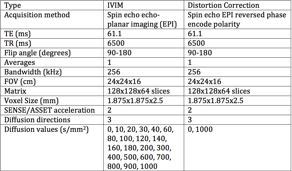
Acquisition:

The protocol contained an IR-SPGR, two identical echo-planar imaging (EPI) IVIM sequences, and a reversed phase encode polarity EPI scan (Table 1). Seven subjects were scanned twice with the same protocol >24 hours apart resulting in 44 separate IVIM acquisitions.

Pre-Processing:

All IVIM scans were EPI-distortion and eddy-current corrected using FSL5 (Topup, Eddy)^6,8. The SRI24 atlas⁹ with 116 regions was registered to the IVIM image via the IR-SPGR image using ANTS¹⁰. SRI24 brain and parcellation masks were transformed to IVIM space and eroded using a 3x3x3 kernel to minimize cross-region and fluid-tissue contamination.

Non-Linear IVIM Fitting:

This method is described elsewhere¹¹, but the fundamentals are that of a two-step fitting where the parameters are guessed using the high and low b-value data separately^1,2 followed by a re-fit using the entirety of the data with the complete bi-exponential model.

Linear IVIM Fitting:

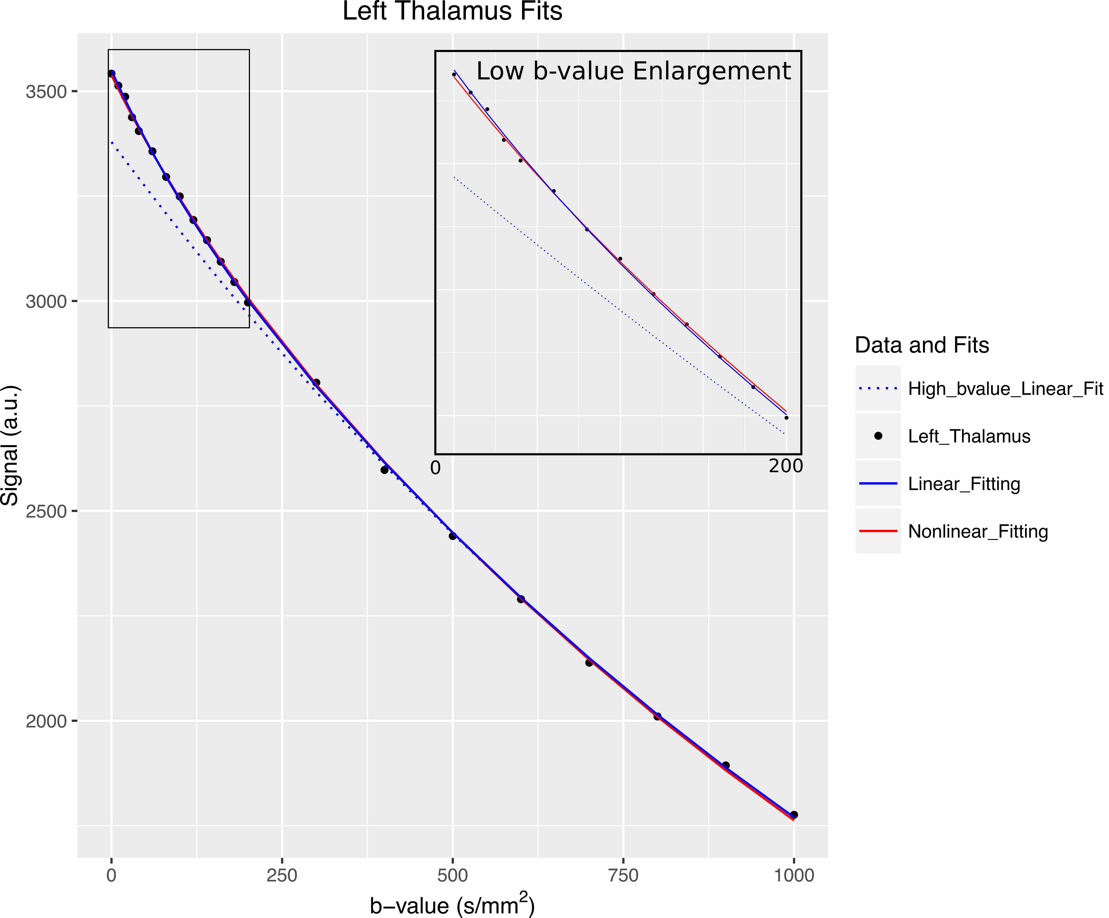
Each region was fit for S0, f, D, D* with S0’, S0* as intermediate variables.

1. Linearly fit ln(S(b>200)) for S0’ and D, where S0’ is the zero intercept of the diffusion fit at b>200.

2. Calculate the residuals for the low b-value data (b<=200) from the fit (data - predicted from step 1).

3. Linearly fit ln(residuals) for S0* and D*, where S0* is the zero intercept of the diffusion fit of the residuals.

4. Calculate S0: S0=S0’+S0*

5. Calculate f as the ratio of the flow signal to the total signal: f=S0*/S0

Both fitting procedures were implemented in Python2.7¹² and produced a single set of IVIM parameters individually for each ROI (Figure 1).

Analysis:

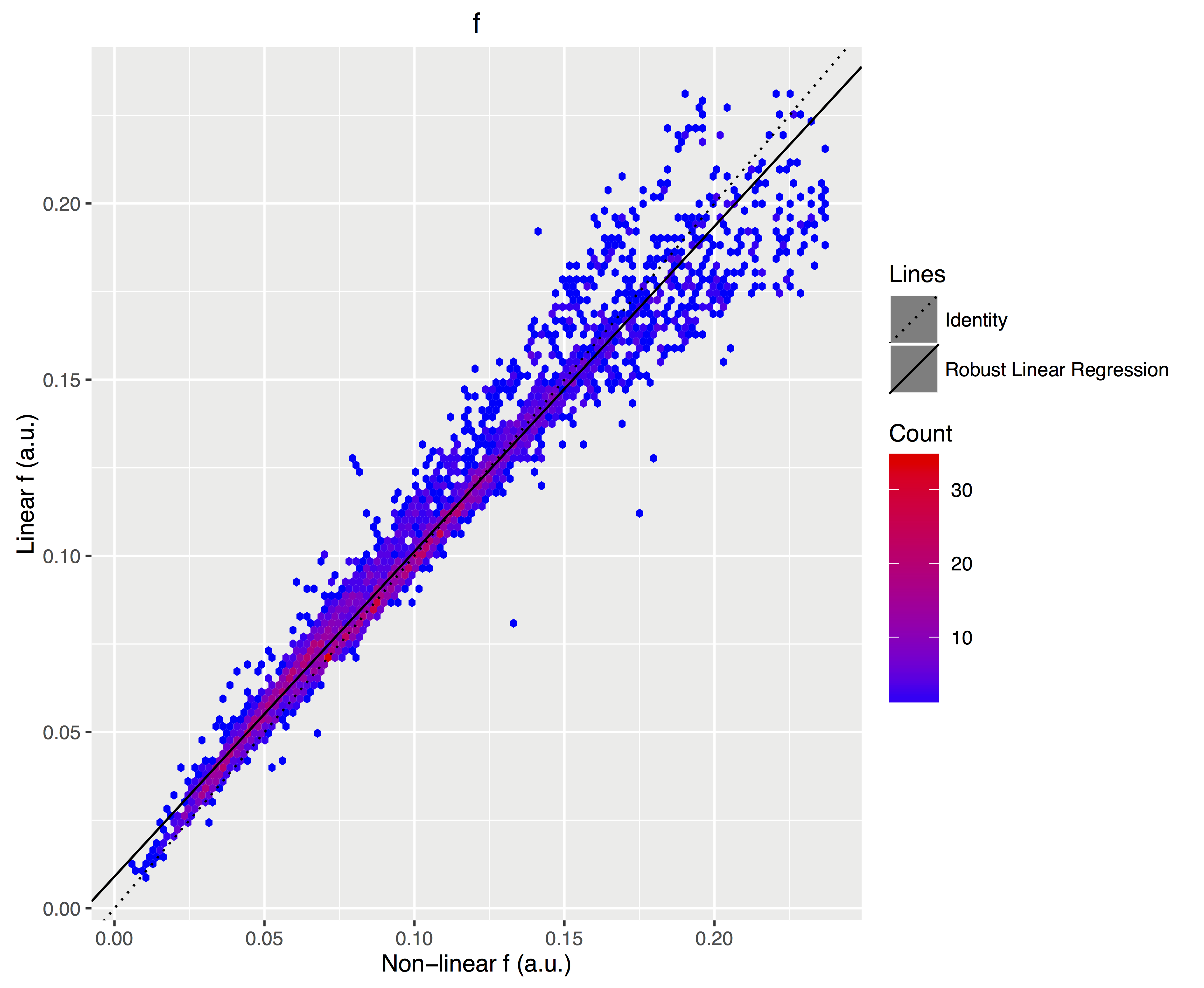
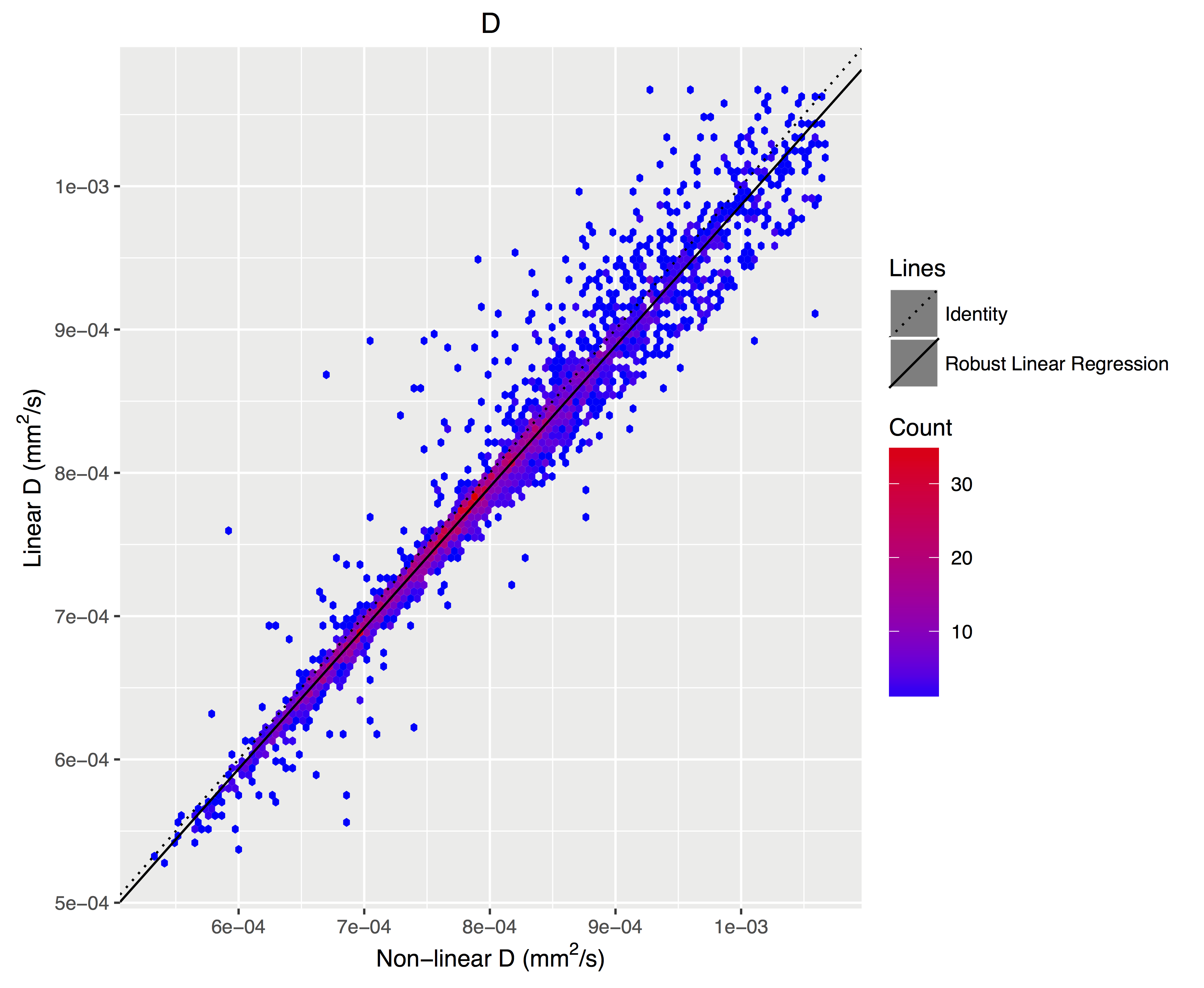
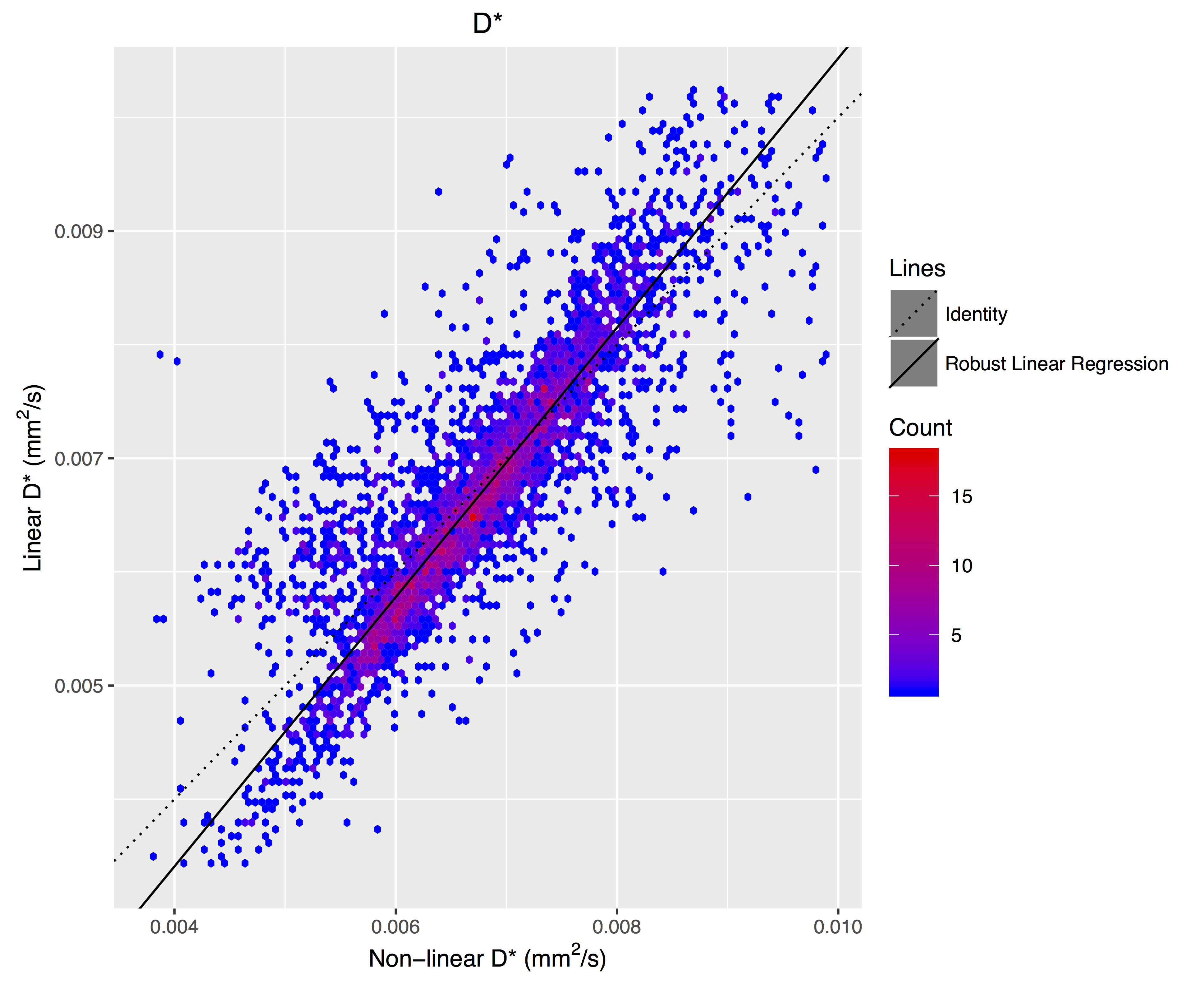
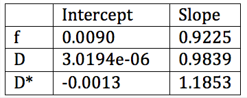
The data cleanup in R¹³ removed nonlinear fits where the region was smaller than 500 mm³ and non-physical values. No cleanup was performed on the matching linear fits. This resulted in 4233 regions fitted with both methods. The best fit regression line on the non-linear versus linear data was calculated using robust regression in order to most accurately capture the overall trend between the fits.

Results

The f (Figure 2), D (Figure 3), and D* (Figure 4) linear fitting values compare very favorably to the nonlinear values (Table 2).

Discussion

Linear fitting takes ~5s to complete for the full 3D IVIM image. This fitting method, while simple, is fast, robust, and compatible with more advanced linear fitting methods such as robust or tensor fitting. Additionally, this method can be used as a fast and accurate starting point for more advanced fitting, such as nonlinear or Bayesian algorithms.

Note that this method is similar to the original method proposed by Le Bihan et al.². However, a major difference is that rather than approximating the combined flow and diffusion compartments with a single exponential, the effect of the diffusion compartment is removed from the data before the flow-only compartment is fit.

The weakness of the proposed method is that it is dependent on the b-value cutoff for the initial fit. This is unavoidable in algorithms that use separate high b-value fitting.

Conclusion

The IVIM metrics are very similar between the traditional nonlinear fit and the proposed linear method. The similarity holds for estimates of f, D, and D*, across a wide range of parameter values and across a large number of brain regions.

Acknowledgements

NIH grants: AA021697, AA021695, AA021692, AA021696, AA021681, AA021690, AA021691, K05 AA017168.

References

1. Federau C, Maeder P, O’Brien K, Browaeys P, Meuli R, Hagmann P. Quantitative Measurement of Brain Perfusion with Intravoxel Incoherent Motion MR Imaging. Radiology. 2012;265(3). doi:10.1148/radiol.12120584.

2. Le Bihan D, Breton E, Lallemand D, Aubin M-L, Vignaud J, Laval-Jeantet M. Separation of diffusion and perfusion in intravoxel incoherent motion MR imaging. Radiology. 1988;168(2):497-505. doi:10.1148/radiology.168.2.3393671.

3. Federau C, Sumer S, Becce F, et al. Intravoxel incoherent motion perfusion imaging in acute stroke: initial clinical experience. Neuroradiology. 2014:629-635. doi:10.1007/s00234-014-1370-y.

4. Gazdzinski S, Durazzo T, Jahng G-H, Ezekiel F, Banys P, Meyerhoff D. Effects of chronic alcohol dependence and chronic cigarette smoking on cerebral perfusion: a preliminary magnetic resonance study. Alcohol Clin Exp Res. 2006;30(6):947-958. doi:10.1111/j.1530-0277.2006.00108.x.

5. Bühler M, Mann K. Alcohol and the human brain: A systematic review of different neuroimaging methods. Alcohol Clin Exp Res. 2011;35(10):1771-1793. doi:10.1111/j.1530-0277.2011.01540.x.

6. Andersson JLR, Skare S. A model-based method for retrospective correction of geometric distortions in diffusion-weighted EPI. Neuroimage. 2002;16(1):177-199. doi:10.1006/nimg.2001.1039.

7. Orton MR, Collins DJ, Koh D-M, Leach MO. Improved intravoxel incoherent motion analysis of diffusion weighted imaging by data driven Bayesian modeling. Magn Reson Med. 2014;71(1):411-420. doi:10.1002/mrm.24649.

8. Smith SM, Jenkinson M, Woolrich MW, et al. Advances in functional and structural MR image analysis and implementation as FSL. Neuroimage. 2004;23 Suppl 1:S208-19. doi:10.1016/j.neuroimage.2004.07.051.

9. Rohlfing T, Zahr NM, Sullivan E V., Pfefferbaum A. The SRI24 multichannel atlas of normal adult human brain structure. Hum Brain Mapp. 2009;31(5):798-819. doi:10.1002/hbm.20906.

10. Avants BB, Tustison NJ, Song G, Cook PA, Klein A, Gee JC. A reproducible evaluation of ANTs similarity metric performance in brain image registration. Neuroimage. 2011;54(3):2033-2044. doi:10.1016/j.neuroimage.2010.09.025.

11. Peterson ET, Zahr NM, Kwon D, Serventi M, Hardcastle C, Sullivan E V. Intra Voxel Incoherent Motion (IVIM) in Brain Regions: a Repeatability and Aging Study. In: Intl. Soc. Mag. Reson. Med. 24. Vol ; 2016.

12. Van Rossum G. Python 2.7, Python Software Foundation. 1991.

13. R Core Team. R Language Definition V. 3.1.1. 2014;3.1.1:55. http://mirror.fcaglp.unlp.edu.ar/CRAN/doc/manuals/r-patched/R-lang.pdf\nhttp://cran.r-project.org/doc/manuals/r-release/R-lang.pdf.

Figures

Table 1: Acquisition parameters for the IVIM and distortion correction reversed phase encode polarity scans.

Figure 1: Signal in the left thalamus with increasing b-values. Nonlinear fitting is shown in red while linear fitting is in blue. The dotted blue line is a linear fit of the high b-values (b>200). The low b-values are enlarged and shown in the insert to highlight the bi-exponential region of the fit. Note that this is a linear fit on the log of the signal so in this plot the raw signal is a mono- or bi-exponential curve.

Figure 2: This binned hexagram plot shows the relationship between f found through nonlinear and linear fitting. Note that the robust linear regression and identity line well describe the relationship between the two fits.

Figure 3: This binned hexagram plot shows the relationship between D found with nonlinear and linear fitting. Because D can be fit linearly from the high b-value data, the dotted identity line and the robust linear fit are almost identical.

Figure 4: This binned hexagram plot shows the relationship between D* found with nonlinear and linear fitting. In this case, the trend is farther from the identity line, but generally follows a straight line that slightly underestimates the lower D* values and overestimates the higher ones. The relationship between the two fitting types is more variable than the other parameters in part because D* is usually only between 3 and 15% of the total signal and is much more susceptible to pulsatile variations during imaging.

Table 2: Shows the intercepts and slopes of the robust regression.

Proc. Intl. Soc. Mag. Reson. Med. 25 (2017)

1767