Purpose

The in-vivo Diffusion MRI (dMRI) signal does not arise from a single diffusion process but instead from the sum of multiple processes. Multi-compartmental modeling requires the knowledge of the compartments and is difficult when the number of exponentials is above 2. In this study we investigate a deconvolution approach to simultaneously estimate non-Gaussian diffusion, free water (FW), IVIM and tissue fractions..

Methods

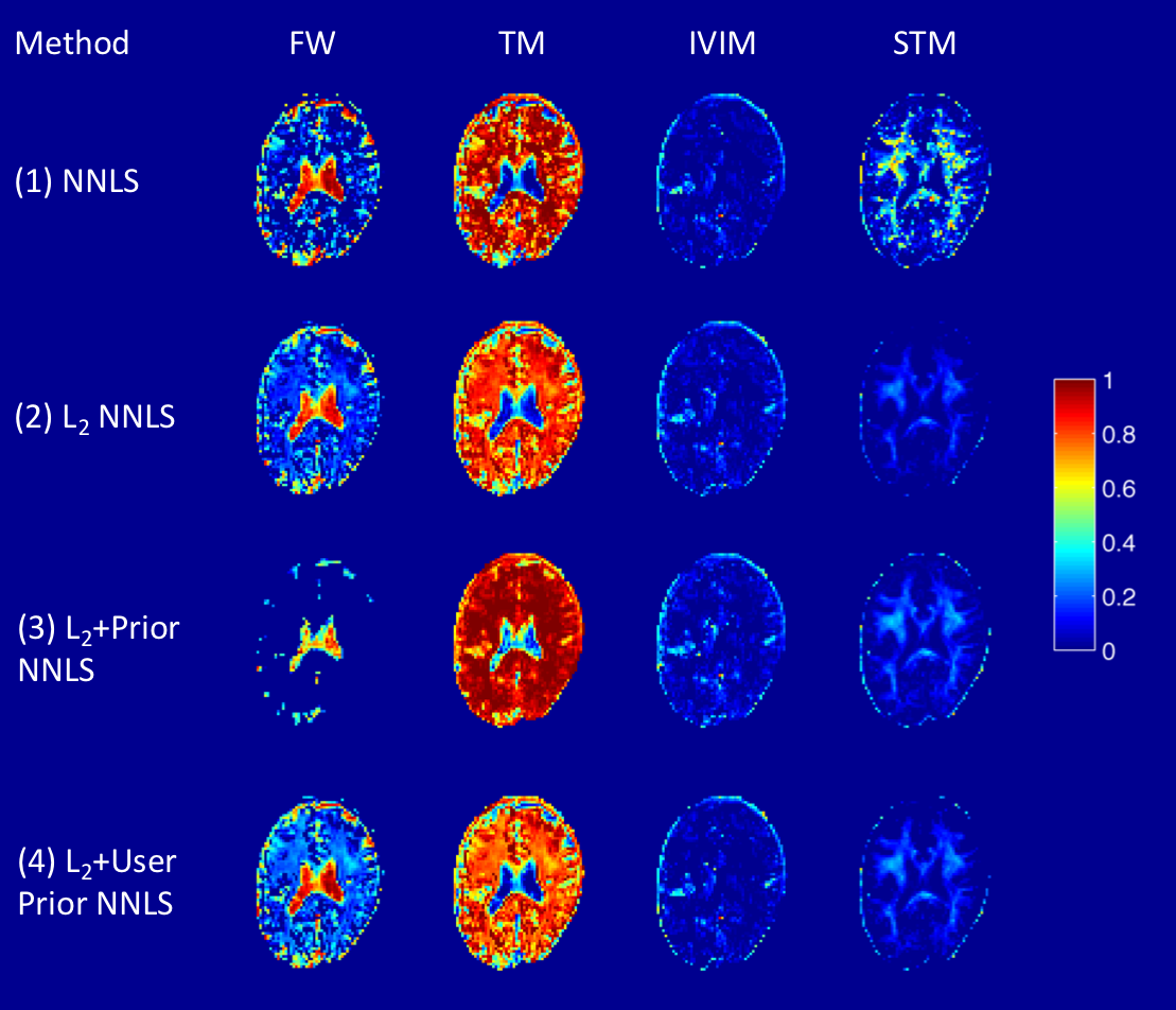
The brain data of a healthy subject was acquired with a 3T scanner. The MRI session included a 1mm³ isotropic T_1W scan, and a dMRI sequence with multiple b-values (resolution 2.5x2.5x2.5mm³). In particular, dMRI included 3 directions for 20 b-values evenly spaced in the b=0-200s/mm² range, 20 b-values evenly spaced in the range b=0-1000s/mm² and 20 b-values evenly spaced in the range b=0-2500s/mm². Pre-processing of the data included b0 drift removal[1] and affine registration of the volumes to the first b=0s/mm²[2]. A deconvolution dictionary was built as collection of 300 Gaussian decaying diffusion signals with log-spaced diffusion coefficients in the range 0.1-1000.0μm²/ms. An additional column corresponding to zero-diffusion was added to the dictionary to account for non-Gaussian diffusion, i.e. to model the plateu of the diffusion signals after restriction effects. The operation was performed with 4 approaches: (1) sparsity promoted non-negative least squares (NNLS), (2) L₂ regularized NNLS[3] (3), L₂ regularized NNLS with data estimated priors and (4) L₂ regularized NNLS with user-imposed prior. Priors for method (3) were computed first averaging the whole brain in a single voxel, to enhance SNR, then computing the whole brain diffusion spectra with NNLS. Priors for step (4) were imposed by assigning non-zero probabilities to diffusion coefficients that can be found in brain dMRI, as 0.6μm²/ms (slow diffusion), 2.0μm²/ms (fast diffusion), 3.0μm²/ms (FW), 10.0μm²/ms (micro-vascular network) and 200.0μm²/ms (vascular network). Fractional maps were computed by integration of the diffusion spectra in specific diffusion ranges: 6.0-1000.0μm²/ms for the IVIM map, 2.5-6.0μm²/ms for the FW map, 0-2.5μm²/ms for the Tissue Map (TM), and 0-0.4μm²/ms for the slow tissue map (STM). T_1W data was segmented with FSL[4], [5] to derive masks of gray matter (GM), white matter (WM) and cerebro-spinal fluid (CSF). Descriptive statistics of the fractional maps were computed to characterize the fractional maps in the three tissues.

Results

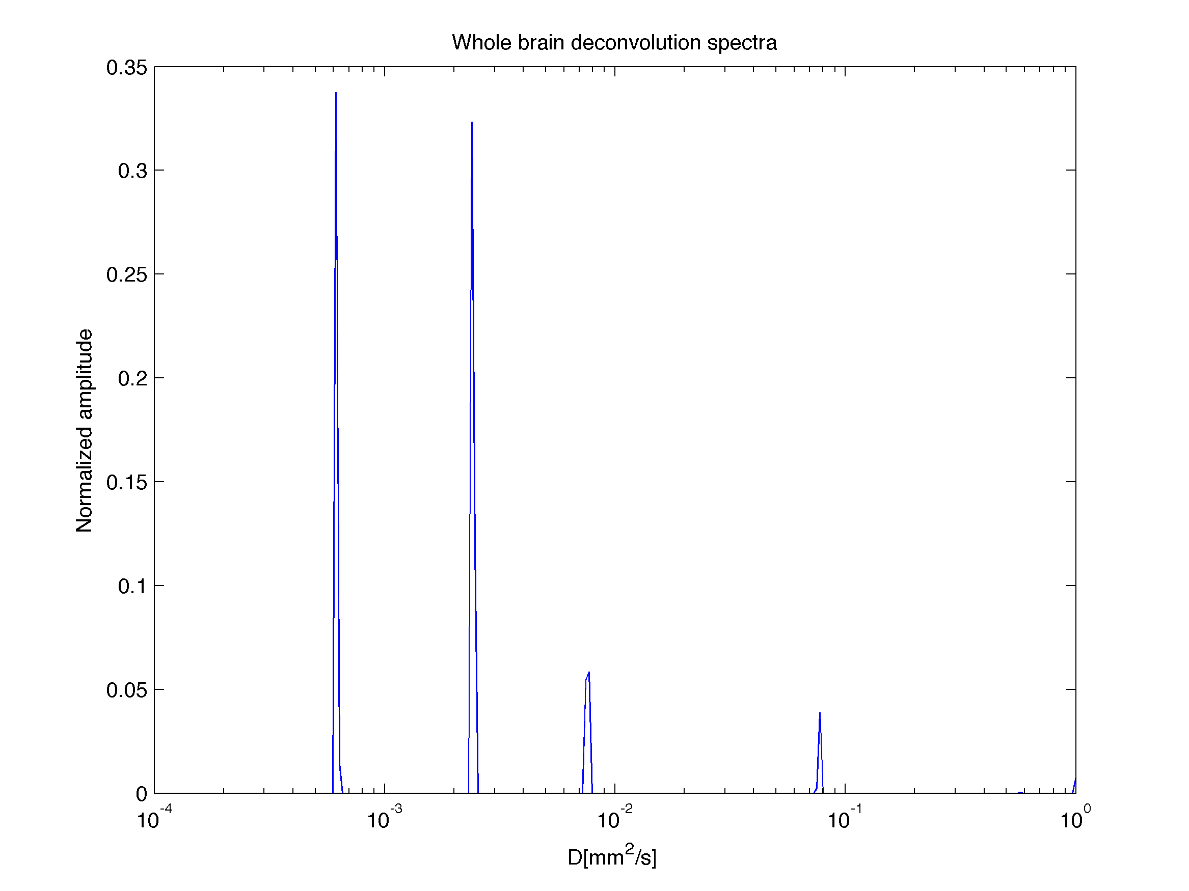
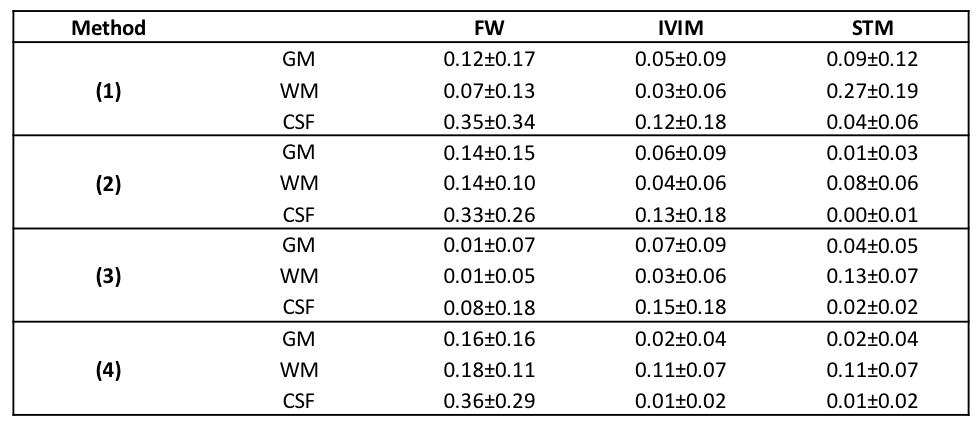
Figure 1 shows the whole brain deconvolution spectra, that was also used as prior for method (3). 5 compartments, corresponding respectively to diffusion coefficients 0.6, 2.4, 7.7, 77.6 and 0μm²/ms (not shown in figure), were revealed. The normalized amplitudes of the peaks were respectively 0.34, 0.32, 0.05, 0.06 and 0.05, therefore the average pseudo-diffusion component was around 10%. Figure 2 shows the fractional maps obtained from the 4 aforementioned methods. Method (1) resulted in the noisiest maps, in particular for STM, while maps from methods (2), (3) and (4) had similar smoothness. FW maps of methods (2) and (4) were similar, and showed higher values than method (3), according to which FW should be zero for most voxels. IVIM maps were consistent across the 4 models. Finally, the STM maps computed with methods (2), (3) and (4) had non-zero values mainly in WM. The mean ± standard deviation of FW, IVIM and STM computed in GM, WM and CSF are reported in Table 1.

Discussion

The four approaches provided consistent results. The IVIM compartment was the most consistent across the four methods, with estimated IVIM between 2 and 13%, and higher values in CSF. The STM maps assumed higher values in WM, in agreement with the design of the dictionary to describe diffusion restrictions The deconvolution spectra computed on the whole volume had 5 peaks (Figure 1), however, the peak corresponding to FW was missing. The method might have failed to disentangle FW from fast diffusion tissue and resulted in an average peak. Even if the method is promising, some limitations should be noted. The choice of the priors is critical, as proved by the comparison of methods (3) and (4). A standardized approach to define the priors should be investigated, as well as the choice of the integration ranges to derive fractional maps.

Conclusions

Regularized deconvolution with priors can be employed to quickly estimate multiple contributions to the measured diffusion signal. Moreover, the method can be used to quickly remove undesired components before quantification with existing tools.

Acknowledgements

No acknowledgement found.