1681
Tradeoffs in pushing the spatial resolution of fMRI for the 7 T Human Connectome Project1Center for Imaging of Neurodegenerative Diseases, Veteran Affairs Health Care System, San Francisco, CA, United States, 2Center for Magnetic Resonance Imaging, University of Minnesota, 3Washington University, 4Oxford Centre for Functional MRI of the Brain, Oxford University
Synopsis
Here we describe subsequent work by the Human Connectome Project (HCP), taking the initial advancements obtained at 3 T and pushing spatial resolution even further at ultrahigh field strengths. To assess the impact of spatial resolution on the resultant detectability of resting state networks throughout the brain, we compare 7 T data acquired at various isotropic spatial resolutions (2 mm, 1.6 mm, 1.5 mm, 1.25 mm, and 0.9 mm) using the 2 mm 3 T HCP rfMRI data as baseline. 7 T functional networks show enhanced BOLD CNR, resulting in sharper, stronger, and more well defined spatial detail even at the group level.
PURPOSE:
High-resolution 7 T fMRI has primarily been constrained to smaller brain regions given the amount of time it takes to acquire enough slices to cover the whole brain at high-resolution. Here we evaluate a range of whole-brain high-resolution resting state fMRI protocols (0.9, 1.25, 1.5, 1.6 and 2 mm isotropic voxels) at 7 T for the Human Connectome Project (HCP). Data were obtained with both in-plane and slice acceleration parallel imaging techniques to maintain the temporal resolution and brain coverage typically acquired at 3 T. The finalized 7 T HCP protocol and data (1.6 mm isotropic, TR=1000ms, IPAT=2, MB=5) have been included in the latest HCP public release: www.humanconnectome.org/documentation/S900.
METHODS:
All data were acquired on a Siemens 7 T Magnetom system, 3 T Trio, or 3 T customized HCP Skyra system using standard 32-channel receive coil arrays. Pilot data for in-depth comparisons of various resolutions and acceleration factors at 7 T was acquired from two non-HCP subjects in five separate scan sessions. One of these subjects was scanned in a sixth scan session with what was later to become the final HCP 7 T fMRI protocol. For comparison of the final HCP 3 T and 7 T protocols, data from an early subset of 24 HCP subjects, scanned at both 3 T and 7 T, were selected for evaluation. For each scan protocol tested, 4 x 15 min resting scans were acquired in which subjects were instructed to rest motionless and awake with their eyes open and fixated on a small fixation cross. All data were pre-processed using the HCP pipeline [1]. ICA-based artifact removal was used to quantify and remove non-neural spatiotemporal components from each 15-minute run of fMRI data [2].RESULTS:
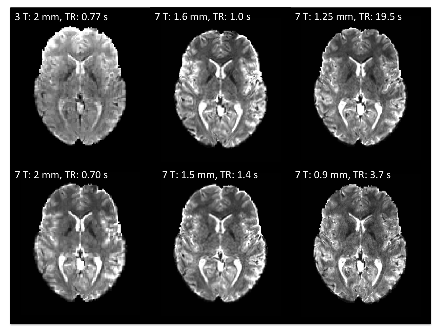
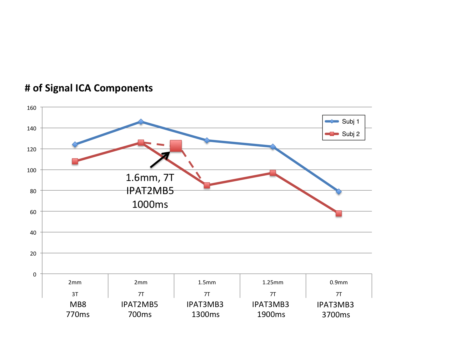
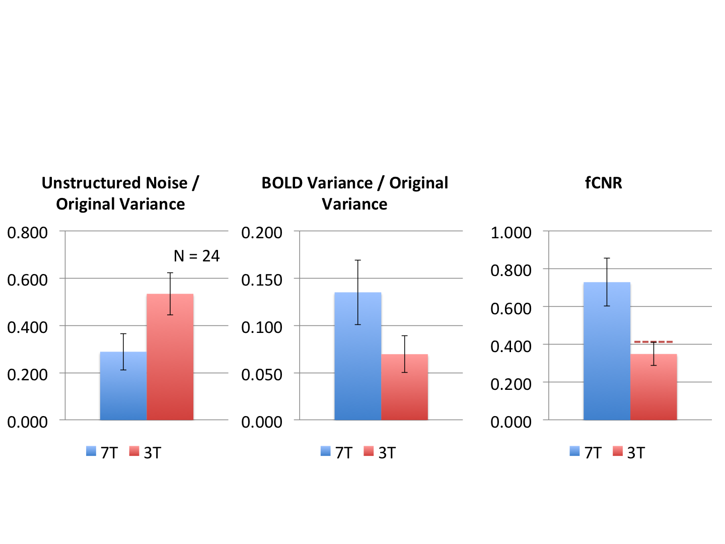
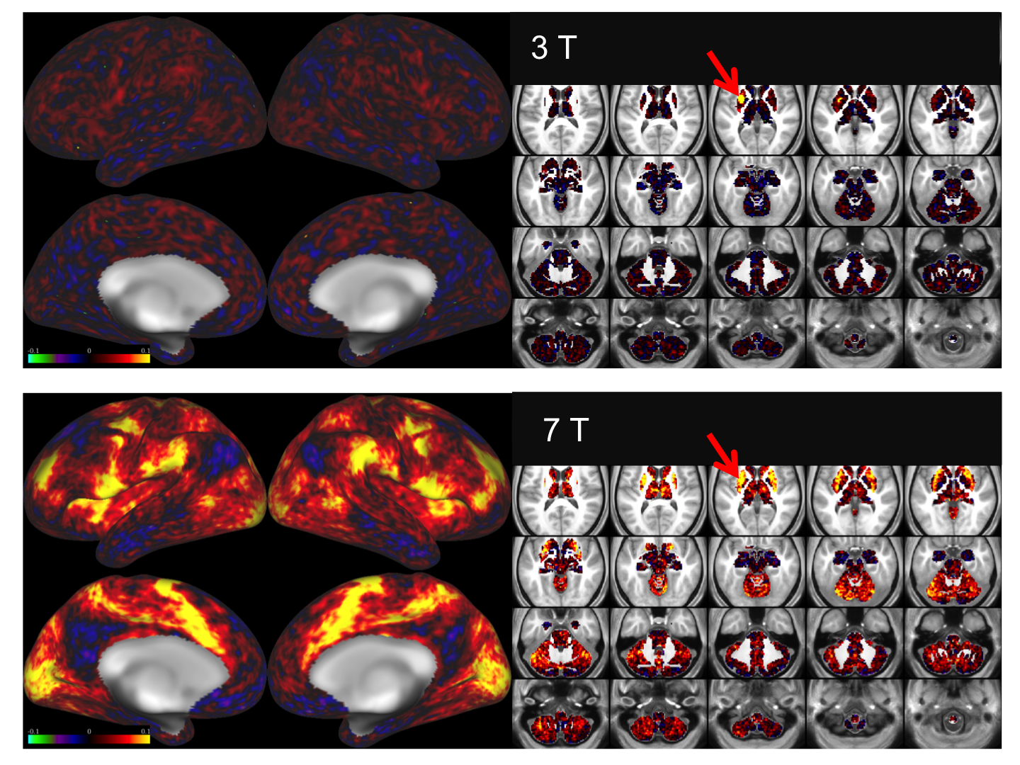
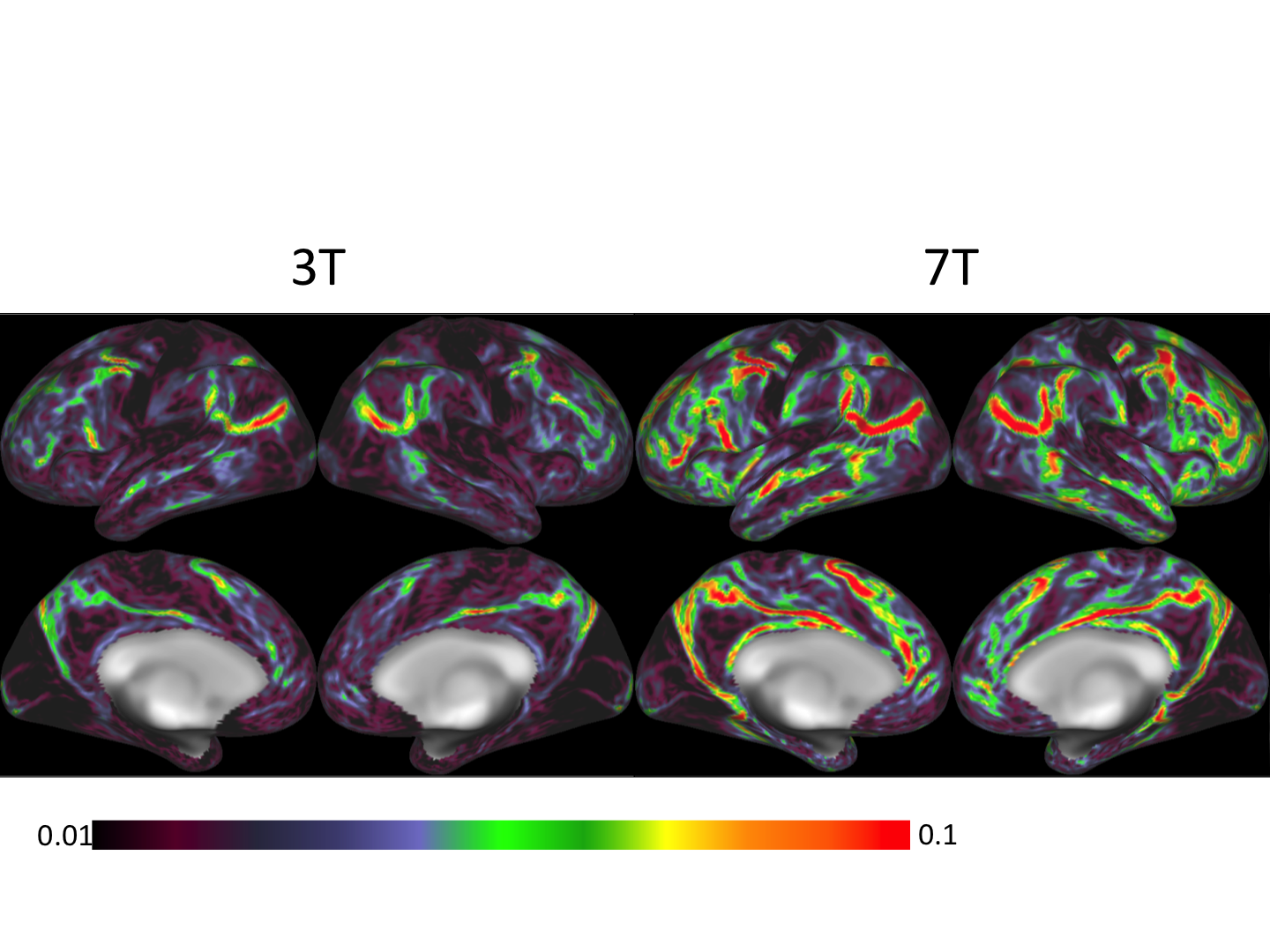
Figure 1 shows representative GE EPI cross sections from a single subject. A) Axial slices. Top row: 3 T 2 mm isotropic (left), 7 T 1.6 mm isotropic (middle) and 7 T 1.25 mm isotropic (right). Bottom row: 7 T 2 mm isotropic (left), 7 T 1.5 mm isotropic (middle), 7 T 0.9 mm isotropic (right). Figure 2 shows the number of resting state signal components as a function of field strength and resolution. Reducing the iPAT factor to 2, was most efficient in terms of TR and SNR per unit time which translated to larger number of detectable signal components. While retaining optimal TE and echo train blurring, a resolution of 1.6 mm was attainable. Figure 3 shows the resting state variance breakdown: 3 T vs 7 T, on average across 24 subjects. Left) Unstructured Noise divided by original variance; where unstructured noise is the residual variance remaining not contributed by the ICA components classified as either “noise” or “signal” (7 T < 3 T; p < 0.05). Middle) BOLD variance divided by original variance; where BOLD variance is the variance contributed by the ICA components classified as “signal” (7 T > 3 T; p < 0.05). Right) Functional contrast to noise ratio (fCNR) as defined as square root of the BOLD variance divided by unstructured noise variance (7 T > 3 T; p < 0.05). Dashed red line indicated fCNR after compensating for difference in number of timepoints sampled in the 7 T and 3 T HCP protocols. Errorbars are STDEV across subjects. Figure 4 shows how reducing partial volume effects at 7 T manifests in terms of dense Connectome connectivity (e.g. correlation coefficient) for an exemplary seed placed in subcortical nucleus, pulvinar (red arrow). Figure 5 shows how the reductions in partial volume effects and increases in fCNR in the 7 T HCP protocol manifests in sharper, stronger, and more well defined dense Connectome connectivity gradients.
CONCLUSIONS:
By taking the initial advancements obtained at 3 T in the HCP and pushing spatial resolution even further at ultrahigh field strengths [3], we demonstrate that high-resolution imaging at the minimum cortical thickness of 1.6 mm can be extended to the entire brain with a temporal resolution of 1 second. Our results suggest that the increased fCNR at 7 T allows for studying resting state networks using voxel volumes half the size as the 3 T HCP protocol (and 37 times smaller than what is conventionally used at 3 T) with significantly less partial volume effects and more distinct spatial features. The improved resolution of the 7 T protocol should allow for robust individual subject parcellations and descriptions of fine-scaled patterns, such as visuotopic organization across cortex.
Acknowledgements
Data were provided by the Human Connectome Project, WU-Minn Consortium(Principal Investigators: David Van Essen and Kamil Ugurbil; 1U54MH091657) funded by the 16 NIH Institutes and Centers that support the NIH Blueprint for Neuroscience Research; and by the McDonnell Center for Systems Neuroscience at Washington University.References
[1] Glasser, M.F., Sotiropoulos, S.N., Wilson, J.A., Coalson, T.S., Fischl, B., Andersson, J.L., Xu, J., Jbabdi, S., Webster, M., Polimeni, J.R., Van Essen, D.C., Jenkinson, M., 2013. The minimal preprocessing pipelines for the Human Connectome Project. NeuroImage 80, 105–124. doi:10.1016/j.neuroimage.2013.04.127
[2] Salimi-Khorshidi, G., Douaud, G., Beckmann, C.F., Glasser, M.F., Griffanti, L., Smith, S.M., 2014. Automatic denoising of functional MRI data: Combining independent component analysis and hierarchical fusion of classifiers. NeuroImage 90, 449–468. doi:10.1016/j.neuroimage.2013.11.046
[3] Ugurbil, K., Xu, J., Auerbach, E.J., Moeller, S., Vu, A.T., Duarte-Carvajalino, J.M., Lenglet, C., Wu, X., Schmitter, S., Van de Moortele, P.F., Strupp, J., Sapiro, G., De Martino, F., Wang, D., Harel, N., Garwood, M., Chen, L., Feinberg, D.A., Smith, S.M., Miller, K.L., Sotiropoulos, S.N., Jbabdi, S., Andersson, J.L.R., Behrens, T.E.J., Glasser, M.F., Van Essen, D.C., Yacoub, E., 2013. Pushing spatial and temporal resolution for functional and diffusion MRI in the Human Connectome Project. NeuroImage 80, 80–104. doi:10.1016/j.neuroimage.2013.05.012
Figures