Synopsis

Gas-free calibration is an appealing new alternative for calibrated fMRI. Using simulations, we determined that estimates of the calibration parameter, M, obtained directly by estimating R₂’ with asymmetric spin echo imaging, are negatively biased. This is due to imperfect spin echo refocusing of spins diffusing in the extravascular space. When we modelled the spin echo attenuation as a quadratic-exponential decay, the imperfect refocusing effects were accurately accounted for over intermediate to large vessel sizes. When tested in vivo, increases in M were observed when using the quadratic model, however, additional sources of decay also contributed to M.

PURPOSE

METHODS - SIMULATIONS

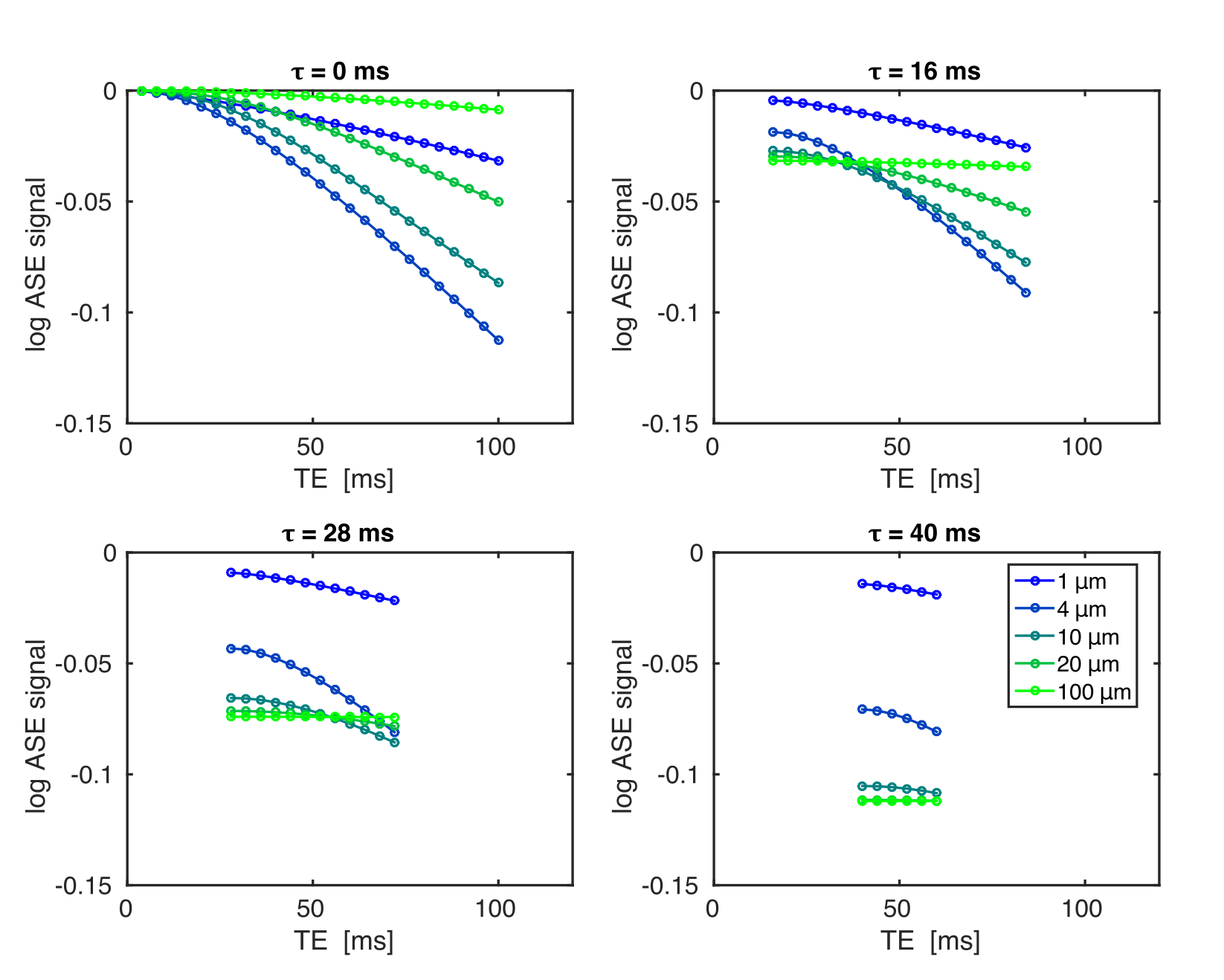
To determine how SE attenuation depends on echo time (TE) and the ASE offset (τ), deterministic simulations of the SE and ASE signals at 3T were run as a function of vessel radius (venous CBV=2%, Hct=40%, SO₂=62%). Fig. 1 shows examples of these simulations. With respect to TE, the curves are all relatively well described by a quadratic-exponential decay early on and by linear-exponential decay later, with the time to transition being proportional to vessel radius.

Ignoring the transition to linear-exponential decay, we propose that the SE attenuation can be described by adding a quadratic-exponential decay with rate constant (R_2,diff)² to the conventional ASE signal description:$$S_{ASE}=S_0e^{-R_2\cdot\text{TE}}e^{-R_2^\prime\cdot\tau}e^{-(R_{2,diff})^2(\text{TE}-\tau)^2}.\quad(1)$$Taking the logarithm of the ratio S_SE/S_ASE gives$$ln\left(\frac{S_{SE}}{S_{ASE}}\right)=ln\left(\frac{S_{ASE}(\tau=0)}{S_{ASE}(\tau)}\right)=R_2^\prime\tau+(R_{2,diff})^2\tau^2-2(R_{2,diff})^2\tau\text{TE}.\quad(2)$$From the linear TE-dependence, it should be possible to estimate (R_2,diff)² and R₂' if this ratio is measured at two or more TEs. M can then be estimated using$$M=e^{R_2^\prime\cdot\text{TE}}-1\simeq R_2^\prime\cdot\text{TE},\quad(3)$$where TE is the echo time of the functional experiment.

METHODS - IMAGING

Pairs of SE and ASE EPI images were acquired at four TEs from 42–70ms in seven healthy subjects at 3T (31 slices, slice thickness=3.5mm, τ=0/30ms, TR=3600ms, FOV=22.4cm, reps=10). Each set of images was acquired at in-plane resolutions of 2.3mm (N=5) and/or 3.5mm (N=5). Field maps were collected to correct for macroscopic through-plane field inhomogeneity-induced decay.

M was estimated with a hypercapnia run of 5% CO₂ (2 min off/on/off). The subjects were imaged with a dual-echo pseudo-continuous ASL sequence to measure the BOLD and cerebral blood flow changes (18 slices, slice thickness=5mm+1mm gap, TR=3600ms, TE₁/TE₂=9.5/30ms, label duration=1600ms, PLD=900ms, FOV=22.4cm, 64x64 matrix). M-estimates were made using a model-based approach with α/β=0.2/1.3.⁵

Comparisons of the M-values from the two techniques were done in each subject’s ASL space using four grey matter (GM) regions of interest (ROIs). M was estimated from the ASE images by averaging the signals within each ROI then calculating M from either ln(S_SE/S_ASE) for the early TE or by using multiple TEs with Eqs. 2 and 3.

RESULTS

Fig. 2 shows simulation results comparing the ideal M (M_ideal), calculated as the maximum possible gradient echo percent BOLD signal at TE=30 ms, to the estimate using ln(S_SE/S_ASE) at a single TE of 40ms (M_ASE), as was done previously,⁴ to the estimate using the quadratic ASE model (q-ASE) with τ=30ms and TEs of 40ms and 50ms (M_q-ASE). M_ASE underestimated M_ideal for all vessel radii, whereas M_q-ASE underestimated M_ideal for small to intermediate radii but was in near perfect agreement with it for radii > ~10 μm.

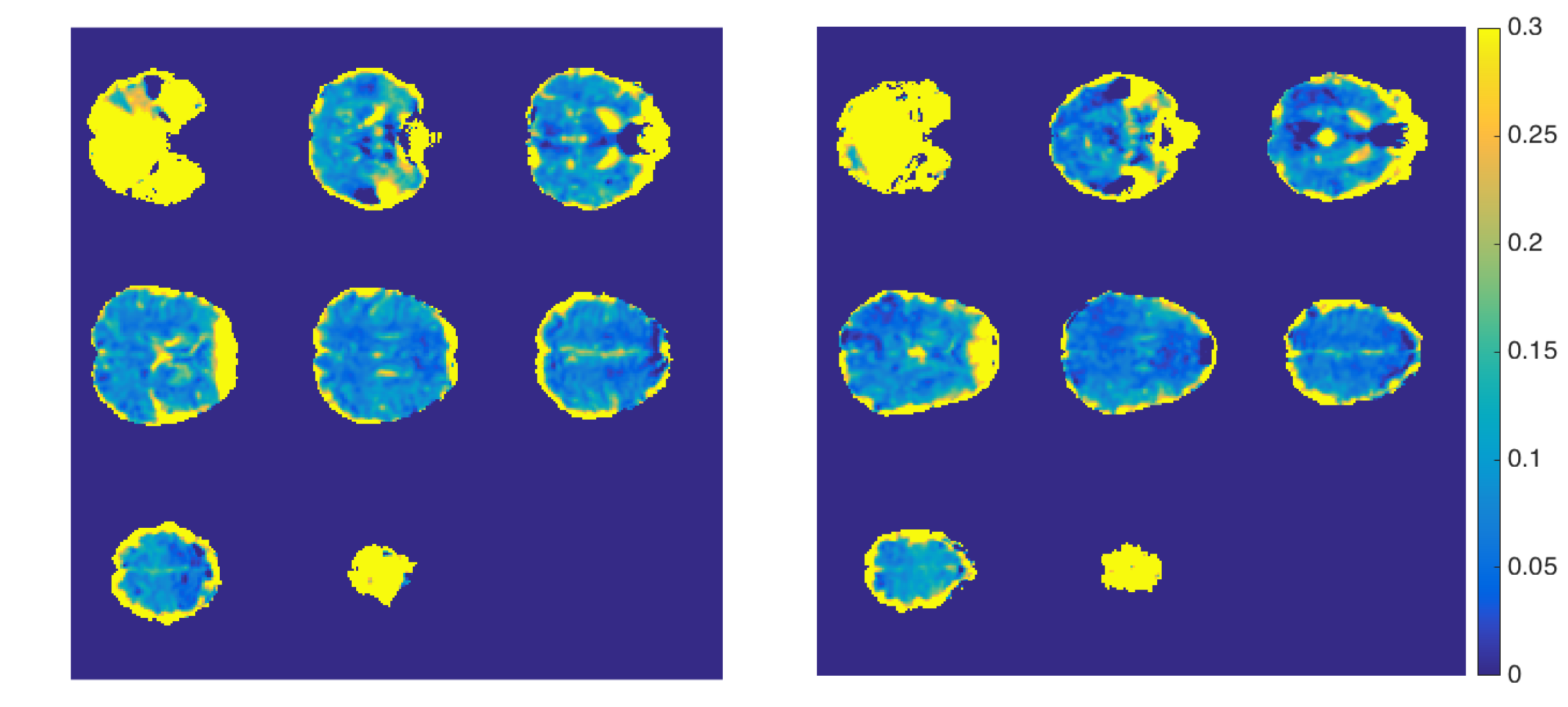
Example M maps from two subjects are shown in Fig. 3. There are hyperintense M-values at the cortical-CSF boundary that likely arise from large blood vessels and CSF.⁶ Because of this, the brain mask used to produce the GM ROIs was eroded to exclude these voxels from analyses where noted.

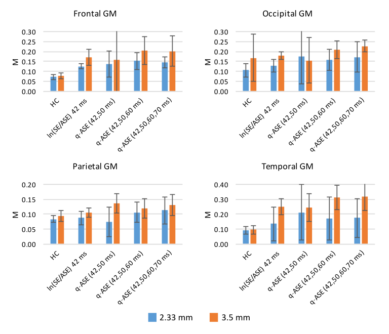
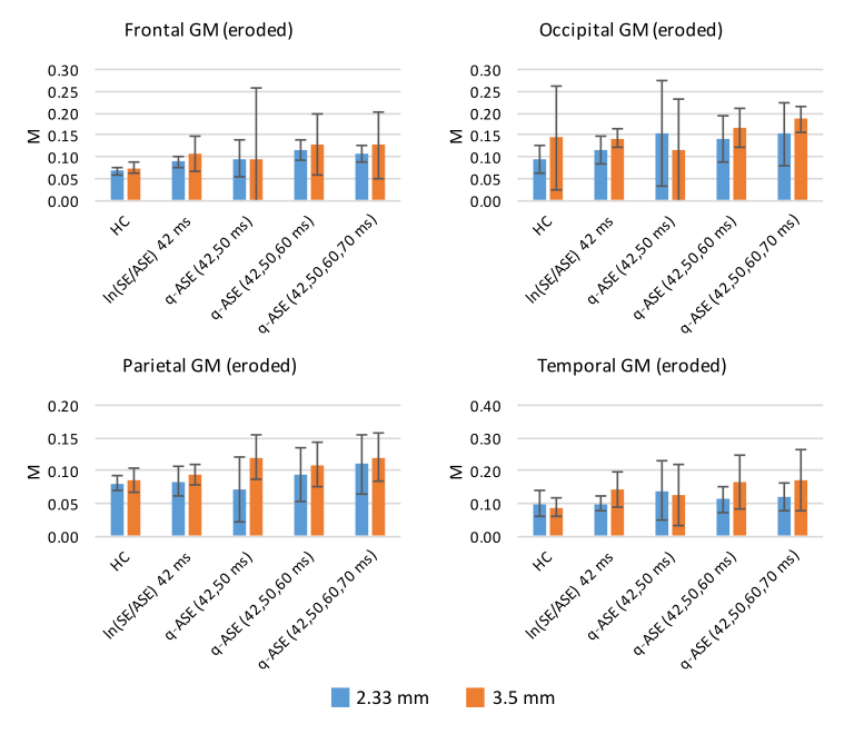
The mean M-values across the ROIs are shown in Figs. 4 and 5 for the original GM ROIs and from the eroded brain mask ROIs, respectively. As expected from the simulations, the in vivo ASE estimates of M were generally found to increase when using the q-ASE model; however, they tended to overestimate the values relative to hypercapnia, in contrast with previous findings.⁴ Increasing the in-plane resolution from 3.5mm to 2.33mm generally decreased the M values, as did using the eroded brain masks. Together, these findings suggest that both macroscopic field gradients and partial voluming with CSF/large blood vessels were important confounding sources of R₂' decay.

CONCLUSION

Acknowledgements

References

[1] T. L. Davis, K. K. Kwong, R. M. Weisskoff, et al. Calibrated functional MRI: mapping the dynamics of oxidative metabolism. PNAS 1998;95(4):1834-9.

[2] P. A. Chiarelli, D. P. Bulte, R. Wise, et al. A calibration method for quantitative BOLD fMRI based on hyperoxia. Neuroimage 2007;37(3):808-20.

[3] N. P. Blockley, V. E. Griffeth, and R. B. Buxton. A general analysis of calibrated BOLD methodology for measuring CMRO2 responses: comparison of a new approach with existing methods. Neuroimage 2012;60(1):279-89.

[4] N. P. Blockley, V. E. Griffeth, A. B. Simon, et al. Calibrating the BOLD response without administering gases: comparison of hypercapnia calibration with calibration using an asymmetric spin echo. Neuroimage 2015;104:423-9.

[5] D. P. Bulte, M. Kelly, M. Germuska, et al. Quantitative measurement of cerebral physiology using respiratory-calibrated MRI. Neuroimage 2012;60(1):582-91.

[6] A. B. Simon, D. J. Dubowitz, N. P. Blockley, et al. A novel Bayesian approach to accounting for uncertainty in fMRI-derived estimates of cerebral oxygen metabolism fluctuations. Neuroimage 2016;129:198-213.