1641
Predicting Diffusion Tensors from Resting-State Functional MRI1Department of Radiology and BRIC, University of North Carolina at Chapel Hill, Chapel Hill, NC, United States, 2Med-X Research Institute, School of Biomedical Engineering, Shanghai Jiao Tong University, Shanghai, People's Republic of China
Synopsis
It has been recently reported that the spatio-temporal correlation of white matter BOLD signals in resting-state functional MRI (rs-fMRI) can be captured using functional correlation tensors (FCTs). FCTs exhibit anisotropy information similar to diffusion tensor imaging (DTI). In this work, we employ a patch-based strategy to improve the noise-robustness of FCTs. Then, we adopt regression forest to learn a mapping from FCTs to DTs. Testing using unseen images, the predicted DTs show high similarity with the actual DTs. This validates the fact that FCTs carries information that is highly correlated with DTs.
Purpose
Functional magnetic resonance imaging (fMRI) measures the blood oxygenation level dependent (BOLD) signals in the gray matter (GM), which is known to be associated with neural activity1. Recently, Ding et al.2 reported that local temporal correlation of BOLD signals in the resting-state fMRI (rs-fMRI) can be found in white matter (WM), reflecting anisotropy similar as diffusion tensors (DTs). They later introduced the functional correlation tensor (FCT)3 to capture this anisotropy. In this work, we improve the noise-robustness of FCTs using a patch-based approach and employ the resulting FCTs for prediction of DTs.Methods
The FCT $$$\boldsymbol{T}_i$$$ for the voxel $$$V_i$$$ in the input fMRI is denoted as a $$$3 \times 3$$$ symmetric matrix written as:
$$\boldsymbol{T}_i= \begin{bmatrix}T_{xx} & T_{xy} & T_{xz} \\T_{xy} & T_{yy} & T_{yz} \\T_{xz} & T_{yz} & T_{zz} \end{bmatrix} .$$
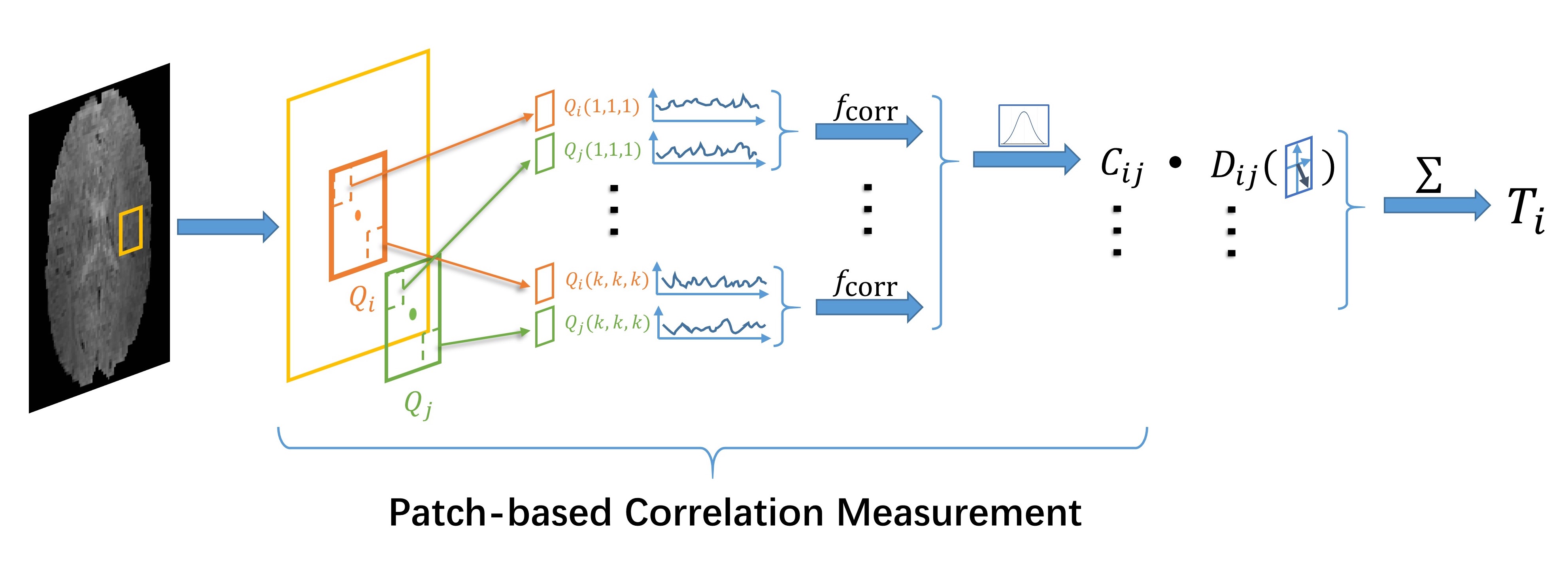
The proposed FCT computed method is illustrated in Fig. 1. For an $$$m \times m \times m$$$ neighborhood window with $$$V_i$$$ as its center voxel, we first compute the Pearson’s correlation coefficients $$$C_{ij}$$$ with all the voxels $$$V_j$$$ within the window. Then, we use a patch-based strategy to measure the correlation coefficients. For two patches $$$Q_i$$$ and $$$Q_j$$$ with the size $$$k \times k \times k$$$, and $$$Q(x,y,z)$$$ represents the voxel in the location $$$(x,y,z)$$$ of the patch $$$Q$$$, we first implement voxel-wise correlation estimation of the two patches, and then fuse the estimates together following a weighted average manner to produce the final result. The equation is given as
$$C_{ij} = \frac{\sum^k_{x=1}\sum^k_{y=1}\sum^k_{z=1}b(x,y,z)~f_{\text{corr}}(Q_i(x,y,z),Q_j(x,y,z))}{\sum^k_{x=1}\sum^k_{y=1}\sum^k_{z=1}b(x,y,z)} ,$$
where $$$f_{\text{corr}}$$$ is the function to compute the Pearson’s correlation coefficient, $$$b(x,y,z)$$$ is the Gaussian kernel given as $$$b(x,y,z)=\exp{(-\frac{(x-\mu)^2+(y-\mu)^2+(z-\mu)^2}{2\rho^2})}$$$, where $$$\mu=(k+1)/2$$$, and $$$\rho$$$ is the scaling coefficient.
We then obtain the unit vector $$$\mathbf{n}_{ij} = \{n_{ij,1},n_{ij,2},n_{ij,3}\}$$$ which describes the direction from $$$V_i$$$ to $$$V_j$$$. The dyadic tensor $$$\mathbf{D}_{ij}$$$ is therefore written as:
$$\mathbf{D}_{ij}=\left(\begin{array}{ccc}n_{ij,1} \cdot n_{ij,1} & n_{ij,1} \cdot n_{ij,2} & n_{ij,1} \cdot n_{ij,3} \\ n_{ij,2} \cdot n_{ij,1} & n_{ij,2} \cdot n_{ij,2} & n_{ij,2} \cdot n_{ij,3} \\ n_{ij,3} \cdot n_{ij,1} & n_{ij,3} \cdot n_{ij,2} & n_{ij,3} \cdot n_{ij,3}\end{array}\right) ;$$
The correlation tensor $$$\boldsymbol{T}_i$$$ is obtained by summing up all the dyadic tensors $$$\mathbf{D}_{ij}$$$ with their corresponding $$$C_{ij}$$$ as the weight coefficients, which is given as:
$$\boldsymbol{T}_i=\sum_j C_{ij}\mathbf{D}_{ij} .$$
Next, we incorporate the regression forest with auto-context model4 to learn the regressor for mapping FCTs to DTs. We use the patch-based strategy5-7 that the regressor maps between the 3D cubic patch of the FCTs, and the corresponding target tensor of DTI in its center voxel. The process consists of the training and testing stages. In the training stage, we randomly select the training patches of the input initial FCTs from the whole brain region. The features are then computed from each patch for training the regressor. The feature extraction process generally follows the work of Zhang et al.7. In the testing stage, every voxel in the whole brain region of the input FCT images are selected. The patches are then extracted, along with the features by following the same settings as in the training stage. The regressor is then applied to compute the mapped tensor estimates.
Results
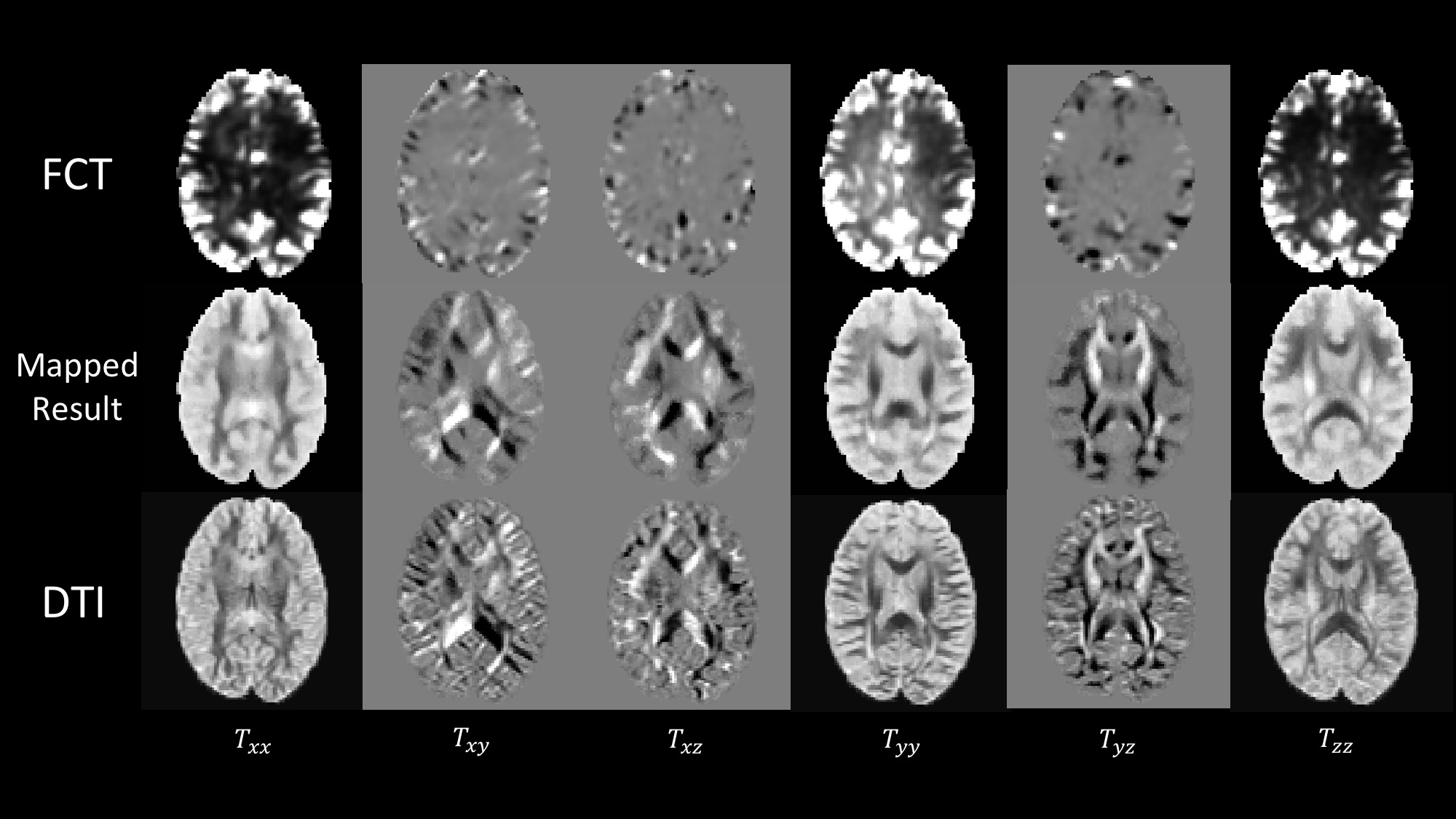
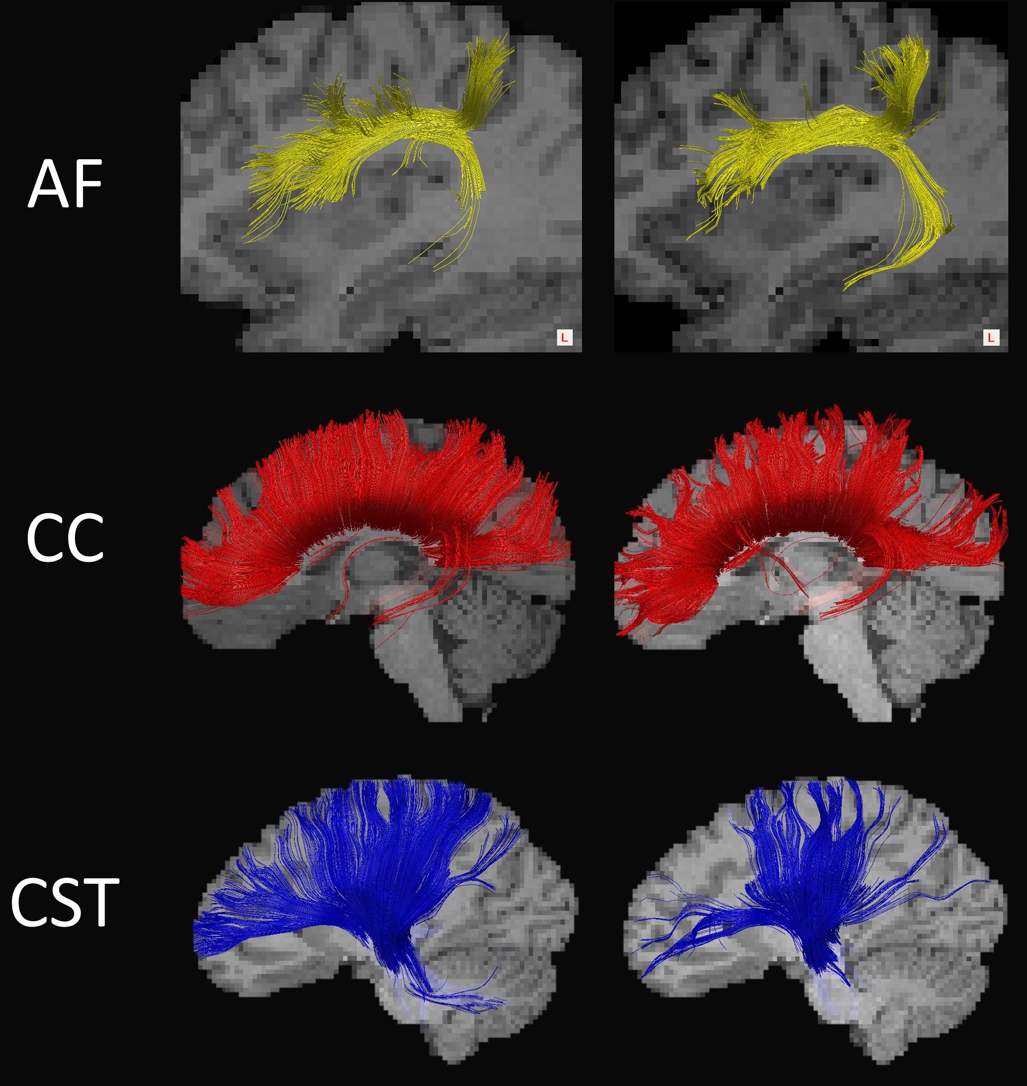
The Human Connectome Project (HCP) dataset is employed to evaluate the performance of the proposed framework. We select 95 subjects from the dataset containing both rs-fMRI and DWI data. We implemented 4-fold cross-validation experiment to produce output tensor maps. Fig. 2 shows six elements of estimated tensor map with DTI as reference. We also present the fiber tracking results for three ROIs in the left hemisphere of the brain in Fig. 3. It can be observed from the figures that the tensors from the regressor has close similarities with DTI data, which clearly demonstrates the direct correspondence between FCT and DTI.Conclusion
We proposed a patch-based approach for improving the noise-robustness of FCTs and use them for DTI prediction.Acknowledgements
This work is supported by National Institutes of Health (NIH) grants (EB006733, EB008374, MH100217, MH108914, AG041721, AG049371, AG042599, AG053867, EB022880).References
1. Honey CJ, Sporns O, Cammoun L, Gigandet X, Thiran J-P, Meuli R, et al. Predicting human resting-state functional connectivity from structural connectivity. Proceedings of the National Academy of Sciences. 2009;106(6):2035-40.
2. Ding Z, Newton AT, Xu R, Anderson AW, Morgan VL, Gore JC. Spatio-temporal correlation tensors reveal functional structure in human brain. PloS one. 2013;8(12):e82107.
3. Ding Z, Xu R, Bailey SK, Wu T-L, Morgan VL, Cutting LE, et al. Visualizing functional pathways in the human brain using correlation tensors and magnetic resonance imaging. Magnetic Resonance Imaging. 2016;34(1):8-17.
4. Tu Z, Bai X. Auto-context and its application to high-level vision tasks and 3D brain image segmentation. IEEE transactions on pattern analysis and machine intelligence. 2010;32(10):1744-57.
5. Zhang L, Wang Q, Gao Y, Wu G, Shen D. Automatic labeling of MR brain images by hierarchical learning of atlas forests. Medical physics. 2016;43(3):1175-86.
6. Zhang L, Wang Q, Gao Y, Wu G, Shen D. Concatenated Spatially-localized Random Forests for Hippocampus Labeling in Adult and Infant MR Brain Images. Neurocomputing. 2016.
7. Zhang J, Zhang L, Xiang L, Shao Y, Wu G, Zhou X, et al. Brain atlas fusion from high-thickness diagnostic magnetic resonance images by learning-based super-resolution. Pattern Recognition. 2016.
Figures