1539
Comparison of T1ρ quantification, SNR, and reproducibility in 3D Magnetization-Prepared Angle-Modulated Partitioned k-space Spoiled Gradient Echo Snapshots (3D MAPSS) and 3D Fast Spin Echo (CubeQuant) techniques.1University of California, San Francisco, San Francisco, CA, United States
Synopsis
Though T2 cartilage mapping has been shown to be sequence dependent, few studies have looked at the inter-sequence variation of cartilage T1ρ quantification. This study compares T1ρ quantification, SNR, and reproducibility of the MAPSS and CubeQuant T1ρ sequences. Four healthy controls received unilateral knee scans. Each patient was scanned twice and was removed from the scanner between scans. Significant differences were found in T1ρ quantification with comparable SNR and reproducibility. This study highlights the importance of using same sequences for quantitative cartilage imaging in multicenter studies.
Purpose
T1ρ and T2 quantitative mapping have been shown to be sensitive to cartilage matrix changes associated with cartilage breakdown.1 Though T2 mapping sequence dependence has been well documented2, few studies have looked at inter-sequence variation of T1ρ quantification. One study compared T1ρ sequences using phantom and specimen scans, however no comparison in human subjects was reported3. The SPGR-based MAPSS T1ρ sequence4,5 (MAPSS) and FSE-based CubeQuant T1ρ sequence6 are two 3D quantitative MRI sequences. Thus, this study compares MAPSS and CubeQuant sequences in terms of T1ρ quantification, signal-to-noise ration (SNR), and reproducibility.Methods
Subjects
Unilateral knee scans were obtained from four healthy volunteers: 2 males and 2 females between 21 and 35 years of age.
Imaging Protocols
MR images were acquired using a 3-Tesla GE MR Scanner (GE Healthcare, MR750 Wide Bore) with an 8-channel phased array knee coil (Invivo). Each subject was scanned twice and removed from the scanner between scans. Imaging parameters are listed in Table 1. These parameters allowed both sequences to take approximately the same time to run.
Image post-processing
Knee cartilage was segmented on the high-resolution 3D-FSE (CUBE) image semi-automatically into six compartments: Medial Femoral Condyle (MFC), Lateral Femoral Condyle (LFC), Medial Tibia (MT), Lateral Tibia (LT), Patella (PAT), and Trochlea (TrF) using an in-house program (Figure 1A). The ROIs were transferred onto the first echo of the first MAPSS scan after registration. The second MAPSS scan and both CubeQuant scans were registered to the first MAPSS scan to ensure the same anatomical regions of cartilage were being compared.7 T1ρ maps were reconstructed using a two-parameter, monoexponential pixel-by-pixel fitting algorithm (Figure 1B). The cartilage was further divided into two even layers, superficial and deep, using an in-house program8 to analyze differences between layers. The goodness of fit for each pixel in the maps was calculated using normalized fitting errors. SNR was calculated on the first echo of MAPSS and CubeQuant images by normalizing the cartilage signal intensity to the noise standard deviation from the background region outside the knee and below the patella as proposed previously.5 The SNR was adjusted for voxel size and square root of acquisition time before comparison between two sequences.
Statistical Analysis
Absolute differences and coefficients of variation (CV) were used to evaluate scan-rescan reproducibility, and paired t-tests were used to analyze differences between MAPSS and CubeQuant quantification.
Results
Overall, excellent reproducibility was attained for both MAPS and CubeQuant sequences (Table 2). The adjusted SNR was higher in MAPSS sequences compared to CubeQuant sequences (Table 3). The normalized fitting error for both sequences was nearly identical with a 0.26 average. CubeQuant showed significantly higher T1ρ values in almost all cartilage compartments (Figure 2), especially in the deep layer. MAPSS had a significantly larger difference between superficial and deep layers than CubeQuant in all compartments (Figure 2).Discussion
Both sequences showed excellent and comparable reproducibility. In the deep layer, MAPSS showed larger CV, primarily due to lower T1ρ values. MAPSS displayed higher adjusted SNR compared to CubeQuant. We acknowledge that due to the spatial variation and non-Gaussian distribution of noise with parallel imaging techniques (as we had in the study), the ROI approach we used was an approximation rather than accurate measurement of SNR. CubeQuant showed significantly higher values than MAPSS, especially in the deep layer. This is potentially due to signal loss of the short T2 component in the CubeQuant sequence with the minimum TE of ~15ms (in contrast, the MAPSS minimum was ~2.5ms), and the blurring at the cartilage-bone interface. Furthermore, the fat suppression was sub-optimal in CubeQuant (Figure 1B), which may also contribute to variation in T1ρ quantification in CubeQuant. With the elevation of T1ρ values in the deep layer, the difference between layers, which has been shown to be a sensitive marker for cartilage degeneration9, is smaller in CubeQuant than MAPSS, suggesting that MAPSS is more sensitive to differences between cartilage layers than CubeQuant.Conclusion
This study showed that MAPSS and CubeQuant sequences perform differently in T1ρ quantification, suggesting that T1ρ mapping is sequence dependent. Thus, for multicenter trials in the future, having the same sequence is critical. Though SNR and reproducibility were comparable, MAPSS may provide more information about cartilage health with its sensitivity to layer differences, while CubeQuant has the advantage of higher resolution (thinner slices with similar scan times).Acknowledgements
This study was supported by GE Healthcare.References
1. Li X, Cheng J, Lin K, Saadat E, et al. Quantitative MRI using T1 ρ and T2 in human osteoarthritic cartilage specimens: correlation with biochemical measurements and histology. Magn Reson Imaging. 2011;29(3):324-34.
2. Pai A, Li X, Majumdar S. A comparative study at 3 T of sequence dependence of T2 quantitation in the knee. Magn Reson Imaging. 2008;26(9):1215-20.
3. Buck FM, Bae WC, Diaz E, et al. Comparison of T1ρ measurements in agarose phantoms and human patellar cartilage using 2D multislice spiral and 3D magnetization prepared partitioned k-space spoiled gradient-echo snapshot techniques at 3 T. AJR Am J Roentgenol. 2011; 196(2):174-9.
4. Li X, Han ET, Busse RF, et al. In vivo T1ρ Mapping in Cartilage Using 3D Magnetization-Prepared Angle-Modulated Partitioned k-space Spoiled Gradient Echo Snapshots (3D MAPSS). Magn Reson Med. 2008;59(2):298-307.
5. Li X, Pedoia V, Kumar D, et al. Cartilage T1ρ and T2 relaxation times: longitudinal reproducibility and variations using different coils, MR systems and sites. Osteoarthritis Cartilage. 2015;23(12):2214-23.
6. Jordan CD, McWalter EJ, Monu UD, et al. Variability of CubeQuant T1ρ, quantitative DESS T2, and cones sodium MRI in knee cartilage. Osteoarthritis Cartilage. 2014;22(10):1559-67.
7. Pedoia V, Li X, Su F, et al. Fully automatic analysis of the knee articular cartilage T1ρ relaxation time using voxel-based relaxometry. J Magn Reson Imaging. 2015; 43(4):970-80.
8. Carballido-Gamio J, Link TM, Majumdar S. New techniques for cartilage magnetic resonance imaging relaxation time analysis: texture analysis of flattened cartilage and localized intra- and inter-subject comparisons. Magn Reson Med. 2008; 59(6):1472-7.
9. Carballido-Gamio J, Stahl R, Blumenkrantz G, et al. Spatial analysis of magnetic resonance T1rho and T2 relaxation times improves classification between subjects with and without osteoarthritis. Med Phys. 2009;36(9):4059-67.
Figures
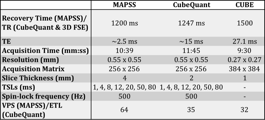
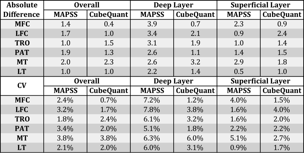
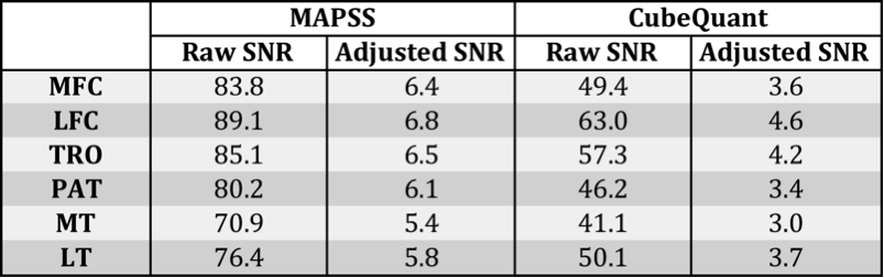
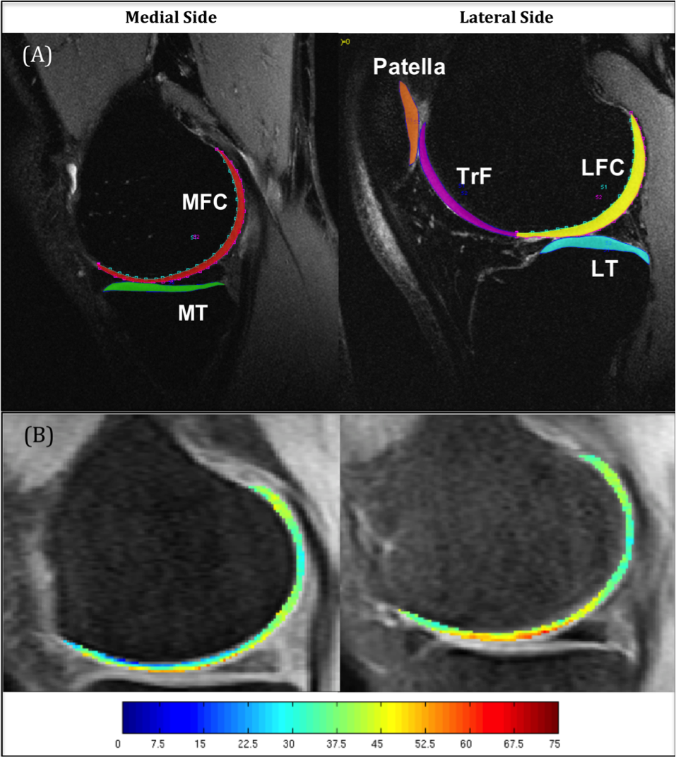
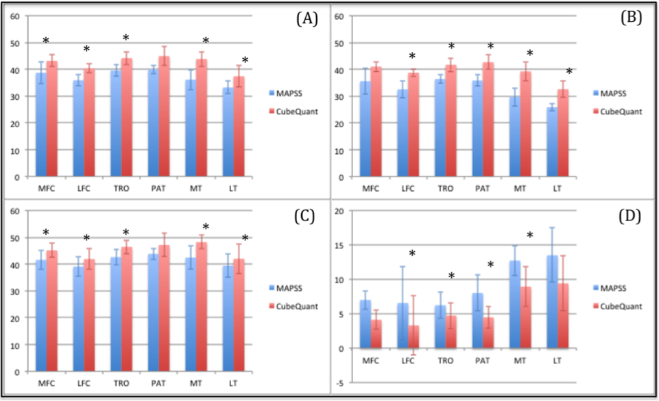
Figure 2. (A) Comparison of T1ρ in the overall cartilage compartments between MAPSS and CubeQuant. (B) Comparison in the deep layer. (C) Comparison in the superficial layer. (D) Absolute difference between deep and superficial layers.
*p < 0.05