1538
Algorithm for Semi-Automatic Segmentation of Hip Acetabular Cartilage Applied to Patients with Femoroacetabular Impingement1Center for Magnetic Resonance Research, University of Minnesota, Minneapolis, MN, United States, 2Consultant, Costa Mesa, CA, United States, 3Radiology, University of Minnesota, Minneapolis, MN, United States, 4Orthopaedic Surgery, University of Minnesota, Minneapolis, MN, United States
Synopsis
A new algorithm to segment the acetabular cartilage based on a single 3D DESS data set is presented. This development was motivated by a need to simplify visualization of 3D quantitative maps of acetabular cartilage damage for surgical planning and arthroscopic correlation. A rapid segmentation algorithm is an important element of this framework, which will be used to guide reparative arthroscopic surgery of patients with femoroacetabular impingement.
Purpose
The integrity of hip acetabulum articular cartilage is an important factor in the clinical management of patients with femoroacetabular impingement (FAI).1 The extent of cartilage damage determines whether a patient is good candidate for reparative arthroscopic surgery. Quantitative mapping of T2*, T2, and T1ρ relaxation times has been proposed to assess the health of the thin, spherical acetabular cartilage.1 An important step in this analysis is presenting this rich 3D quantitative information in a simple manner to the orthopaedic surgeon for surgical planning. To address this need, we developed a post-processing pipeline 2 that (i) segments the acetabular cartilage from a high-resolution 3D dual echo steady state (DESS) acquisition, (ii) registers a quantitative map to the 3D DESS data set, (iii) assigns relaxation times to the segmented acetabular cartilage, and (iv) flattens the quantitative 3D cartilage surface with a standard orientation, resulting in a simplified 2D display. The rate-limiting step of this pipeline is the cartilage segmentation, which is currently done manually. In this work, we present a new semi-automatic algorithm to dramatically reduce the time needed to segment the acetabular cartilage using a single 3D DESS data set. To validate the approach, algorithm and manual segmentations were compared using 3D DESS data sets acquired for patients with FAI.Methods
Test Data. 3D DESS images of a unilateral hip were clinically acquired for a series of patients with FAI using a Siemens 3T MRI system and a matrix flex coil. 3D DESS sequence parameters were: FOV=20×20×8 cm3; matrix=256×256×128; TR/TE=12.3/4.9 ms; flip angle=28°; and BW=325 Hz/px. For segmentation, the 3D DESS images were loaded into BrainVoyager QX 3 and interpolated to 0.4 mm isotropic spatial resolution with a 2563 voxel bounding box centered on the femoral head.
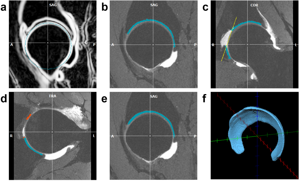
Segmentation Algorithm. The acetabular cartilage segmentation algorithm was developed as a BrainVoyager QX plugin. First, the femoral head surface is automatically detected using spherical edge detection (Figure 1a). Second, edge-based thresholding is used to define the boundaries of the acetabular cartilage based on assumed signal ratio differences between bright cartilage and dark bone, edge detection of the neighboring femoral head articular cartilage, and proximity to the femoral head surface (Figure 1b). These boundaries are defined along radial lines extending from the center of the femoral head and projecting orthogonally to the cartilage surface. Default parameters for the edge detection were derived empirically from a series of test data sets. These default parameters enable automatic detection of the acetabular cartilage; alternatively, the parameters can be manually modified, with graphical feedback, to fine-tune the segmentation on a per-subject basis. Third, the acetabular fossa fat pad is removed by defining a cut plane through the spherical surface (Figure 1c). An initial guess is made for the cut plane position, but it must then be manually adjusted. Fourth, the transverse ligament is removed by automatically detecting it at the notch of the acetabular cartilage and then manually adjusting its extent to where it abuts the acetabular cartilage (Figure 1d). Fifth, the segmentation is smoothed (Figure 1e). Lastly, a vector along the transverse ligament and an orthogonal vector pointing to the most distant aspect of the femoral head sphere are used to define a standard orientation to guide the surgeon.
Validation Study. The acetabular cartilage for three 3D DESS test data sets that were not used in the development of the algorithm were segmented both manually (by a musculoskeletal radiologist) using ITK-SNAP 4 and semi-automatically (by a different person) using the algorithm. The algorithm was performed using default parameters. The resultant segmentations were compared numerically in Matlab using the Dice similarity metric and qualitatively by visual comparison in Paraview.5
Results
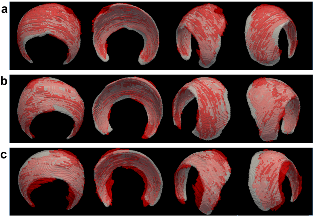
The average time to complete the manual segmentations was 120 minutes, whereas the semi-automatic segmentations only required <3 minutes. The algorithm produced results very similar to the manual segmentations. The Dice similarity coefficients for the three segmentations were 0.75, 0.77, and 0.70, which suggest a strong similarity between the manual and semi-automatic segmentations when compared to prior work with articular cartilage segmentations.6-8 Visual comparisons between the manual and semi-automatic segmentations are shown in Figure 2.Discussion
The new algorithm provides a rapid means to segment the acetabular cartilage for improved visualization of rich 3D quantitative information or subsequent analyses. The algorithm performed well with default parameters, and the program flexibly allows user control to refine results on a per-subject basis if desired. This algorithm is an important step toward realizing quantitative-mapping-guided surgical planning in routine clinical practice.Acknowledgements
We thank Rainer Goebel for assistance with the BrainVoyager QX plugin development. This study was supported in part by the NIH (P41 EB015894).References
1. Riley GM, McWalter EJ, Stevens KJ, Safran MR, Lattanzi R, Gold GE. MRI of the hip for the evaluation of femoroacetabular impingement; past, present, and future. J Magn Reson Imaging 2015; 41(3):558-72.
2. Ellermann J, Ziegler C, Nissi MJ, Goebel R, Hughes J, Benson M, Holmberg P, Morgan P. Acetabular cartilage assessment in patients with femoroacetabular impingement by using T2* mapping with arthroscopic verification. Radiology 2014; 271(2):512-23.
3. Goebel R, Esposito F, Formisano E. Analysis of functional image analysis contest (FIAC) data with Brainvoyager QX: From single-subject to cortically aligned group general linear model analysis and self-organizing group independent component analysis. Human Brain Mapping 2006; 27:392-401.
4. Paul A. Yushkevich, Joseph Piven, Heather Cody Hazlett, Rachel Gimpel Smith, Sean Ho, James C. Gee, and Guido Gerig. User-guided 3D active contour segmentation of anatomical structures: Significantly improved efficiency and reliability. Neuroimage 2006; 31(3):1116-28.
5. Ahrens J, Geveci B, Law C. ParaView: An End-User Tool for Large Data Visualization. Visualization Handbook, Elsevier, 2005.
6. Neubert A, Yang Z, Engstrom C, Xia Y, Strudwick MW, Chandra SS, Fripp J, Crozier S. Automatic segmentation of the glenohumeral cartilages from magnetic resonance images. Med Phys 2016; 43(10):5370.
7. Ozturk CN, Albayrak S. Automatic segmentation of cartilage in high-field magnetic resonance images of the knee joint with an improved voxel-classification-driven region-growing algorithm using vicinity-correlated subsampling. Comput Biol Med 2016; 72:90-107.
8. Pang J, Li P, Qiu M, Chen W, Qiao L. Automatic articular cartilage segmentation based on pattern recognition from knee MRI images. J Digit Imaging 2015; 28(6):695-703.
Figures