1512
Strategies for Compensating for Missing k-space Data in a Novel Half-Fourier ReconstructionSeul Lee1 and Gary Glover2
1Electrical Engineering, Stanford University, Stanford, CA, United States, 2Radiology, Stanford University, Stanford, CA, United States
Synopsis
Functional MRI (fMRI) is sensitive to off-resonance from air-tissue susceptibility interfaces. Existing half-Fourier reconstruction is vulnerable to off-resonance since it may lose most of the image energy (near k=0) with a large amount of off-resonance. In a previous study, we suggested a new half Fourier (even/odd (E/O)) reconstruction and showed it was more robust to off-resonance compared to Homodyne reconstruction. E/O reconstruction acquires every other line in k-space. Therefore, neighboring data can be used to compensate for the missing data. In this study, we suggest several strategies for compensating for missing k-space data in kx-ky as well as kz direction.
Introduction
Since a real object has Hermitian symmetric property, only half of k-space is required to reconstruct images. Homodyne1 is a well-known reconstruction method to acquire half of k-space and a few additional k-space data at the center to overcome phase shifts. However, it is vulnerable to off-resonance. We introduced a new method for half Fourier reconstruction (even/odd (E/O) reconstruction) in a previous study. E/O reconstruction acquires even lines of the left half, odd lines of the right half and additional full k-space lines at the center (same number of lines as those of homodyne) (Fig. 1). In Homodyne reconstruction, acquired half of k-space data can be used to complement the rest of the half of k-space. In E/O reconstruction, however, a few other methods can be applied to compensate for missing data. In this study, we suggest several methods to complement missing k-space data caused by half Fourier acquisition in E/O reconstruction: 1) neighboring samples in each 2D k-space line and 2) neighboring 3D kz lines. Compared to Homodyne reconstruction that requires phase correction, the strategies that we suggest do not require any phase correction.Methods
Data Acquisition: With IRB approval, we scanned a human brain using a 2D EPI sequence with 150 timeframes to evaluate five different methods to compensate for missing data. Data were acquired using a 3T GE whole-body MRI scanner equipped with a single-channel RF receive coil and a single-shot gradient-echo sequence with TE/TR=30/2000 ms, 3.4 mm x 3.4 mm x 4 mm voxels, FOV=22 cm×22 cm, 10 slices, BW=484 Hz/pixel, flip angle=77 degrees and scan time=5 min. Image Reconstruction: For half Fourier reconstruction, we acquired full k-space data and padded zeros in half of k-space. We compared five methods for compensating for missing data in terms of reconstructed images, difference images between each reconstructed images and the reconstructed image from full k-space data and temporal SNR (tSNR). For tSNR, the 6th slice was chosen, and the average tSNR of that slice (non-zero voxels only) was calculated. The five methods are: 1) linear interpolation, 2) mean of six neighboring samples, 3) GeneRalized Autocalibrating Partially Parallel Acquisitions (GRAPPA)2 method using neighboring samples, 4) mean of twelve samples in neighboring kz lines, and 5) GRAPPA method using neighboring kz lines. 1), 2) and 3) are the methods that compensate for missing data using neighboring samples in each slice (2D neighbors, Fig. 2) and 4), 5) are the methods that compensate using neighboring kz lines (3D neighbors). For GRAPPA method, we calculated coefficients from the center that are fully acquired and applied those coefficients to fill missing samples and alternative lines were acquired in each slice for 3D GRAPPA (e.g. previous slice has alternative lines compared to current slice) (Fig. 3).Results
Five different compensating methods reconstructed images successfully though air-tissue interface such as frontal lobe and sinuses were attenuated due to different effects of susceptibility (Fig. 4). From the difference image between reconstructed images from five methods and those from full k-space data, the reconstructed images from 1) linear interpolation, 2) mean of six neighboring samples, 4) mean of twelve samples in neighboring kz lines showed similar results, however, that from GRAPPA method, both 2D and 3D, showed larger difference from the images of full k-space data compared to other methods. In terms of average tSNR of the 6th slice compared to the reconstructed image from fully sampled data, 1) interpolation showed 75.5%, 2) mean of six neighboring samples showed 76.6%, 3) GRAPPA method (2D) showed 97.9%, 4) mean of twelve samples in neighboring kz lines showed 86.1% and 5) GRAPPA method (3D) showed 97.7%. tSNR maps are shown in Fig. 5. In the 2D case, methods 1 and 2 demonstrated tSNR very close to that expected from subsampling, 75.6%.Discussion
We filled missing data using Hermitian symmetry and it showed attenuation. This is because MR data in practice are not real and it contains off-resonance. Therefore, phase correction must be applied in this case. However, all the five methods that we suggested reconstruct images successfully without phase correction. Phase correction must be applied for Homodyne reconstruction, however, we demonstrate there are several compensating methods with which phase correction is not required for E/O reconstruction. Among those methods, less signal dropout was observed in 1) linear interpolation and 2) mean of six neighboring samples although with slightly reduced tSNR.Acknowledgements
We thank Haisam Islam for the EPI sequence. Funding for this work was provided by: NIH EB015891References
1. Homodyne detection in magnetic resonance imaging. Noll D.C et al., Medical Imaging, IEEE Transactions on, 10(2):154-163,1991 2. Generalized Autocalibrating Partially Parallel Acquisitions (GRAPPA). Griswold et al., Magnetic Resonance in Medicine, 47(6):1202-1210, 2002Figures
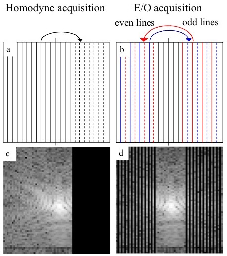
Figure 1. (a) Homodyne method acquires half
lines and additional lines at the center, (b) E/O method acquires odd lines of
half, even lines of the rest of half and full lines at the center. (c) and (d)
are the k-space data from both acquisition methods, respectively (shown in log
scale).
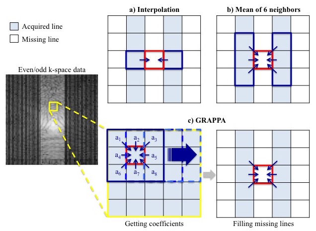
Figure 2.
Left image shows k-space data from E/O reconstruction,
(a)-(c) shows how to fill missing data using neighboring samples (2D): (a)
interpolation, (b) mean of six neighboring samples, and (c) GRAPPA. Blue
colored and white voxels correspond to acquired and not-acquired samples,
respectively.
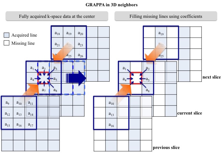
Figure 3. GRAPPA method for filling missing data using
neighboring kz lines (3D). Blue colored and white voxels correspond to acquired
and not-acquired samples, respectively. Coefficients are calculated at the
center, and missing samples are filled using those coefficients. Each slice has
alternatively acquired lines.
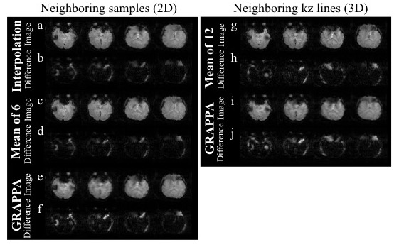
Figure 4.
Reconstructed images (a, c, e, g and i) and difference
images (b, d, f, h and j) between reconstructed image from full k-space data
and reconstructed images from five methods: 1) interpolation (a, b), 2) mean of
six neighboring samples (c, d), 3) GRAPPA (2D) (e, f), 4) mean of twelve
neighboring kz lines (g, h), 5) GRAPPA (3D) (i, j).
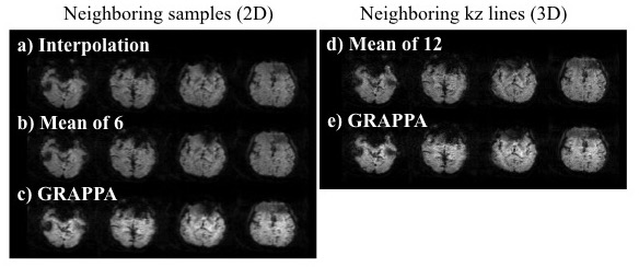
Figure 5.
tSNR of the reconstructed images from five methods: 1)
interpolation (a), 2) mean of six neighboring samples (b), 3) GRAPPA (2D) (c),
4) mean of twelve neighboring kz lines (d), 5) GRAPPA (3D) (e).