1505
Spatial Mapping Using Radio Frequencies: A Non-Linear Approach to Silent MRI1University of California Irvine, Irvine, CA, United States, 2University of California Berkeley, Berkeley, CA, United States
Synopsis
Recent advances for silent MRI have shown that spatial encoding can be achieved using RF rather than linearly varying static magnetic field gradients. This has been demonstrated using homogeneous transmit (B1) fields with linearly varying phase gradients. Similar results can be achieved with linear B1 amplitude gradients with homogeneous phase. The efficacy of either method is limited by a maximum B1 gradient strength (phase or magnitude) per specific absorption rate. Here we demonstrate a novel approach to relieve this restriction where highly nonlinear B1 gradients can be used for combined amplitude and phase modulation with reconstruction using state-of-the-art machine learning models.
Introduction
Magnetic resonance imaging (MRI) methods use non-ionizing radiation in combination with a large static magnetic field to probe the magnetic properties of biological tissue. Current MRI methods rely on the use of linearly varying static magnetic fields generated by gradient coils to spatially encode the MRI signal. The utility of MRI is limited by these gradients causing high levels of acoustic noise and peripheral nerve stimulation (PNS). This work reports a novel MRI method that entirely eliminates both acoustic noise and PNS by transferring the burden of spatial encoding from acoustically loud gradient coils to silent radio frequency (RF) devices. Achieving spatial mapping of the MR signal using highly parallel radio frequency transmitters and receivers, rather than gradient fields, lies at the core of this approach.
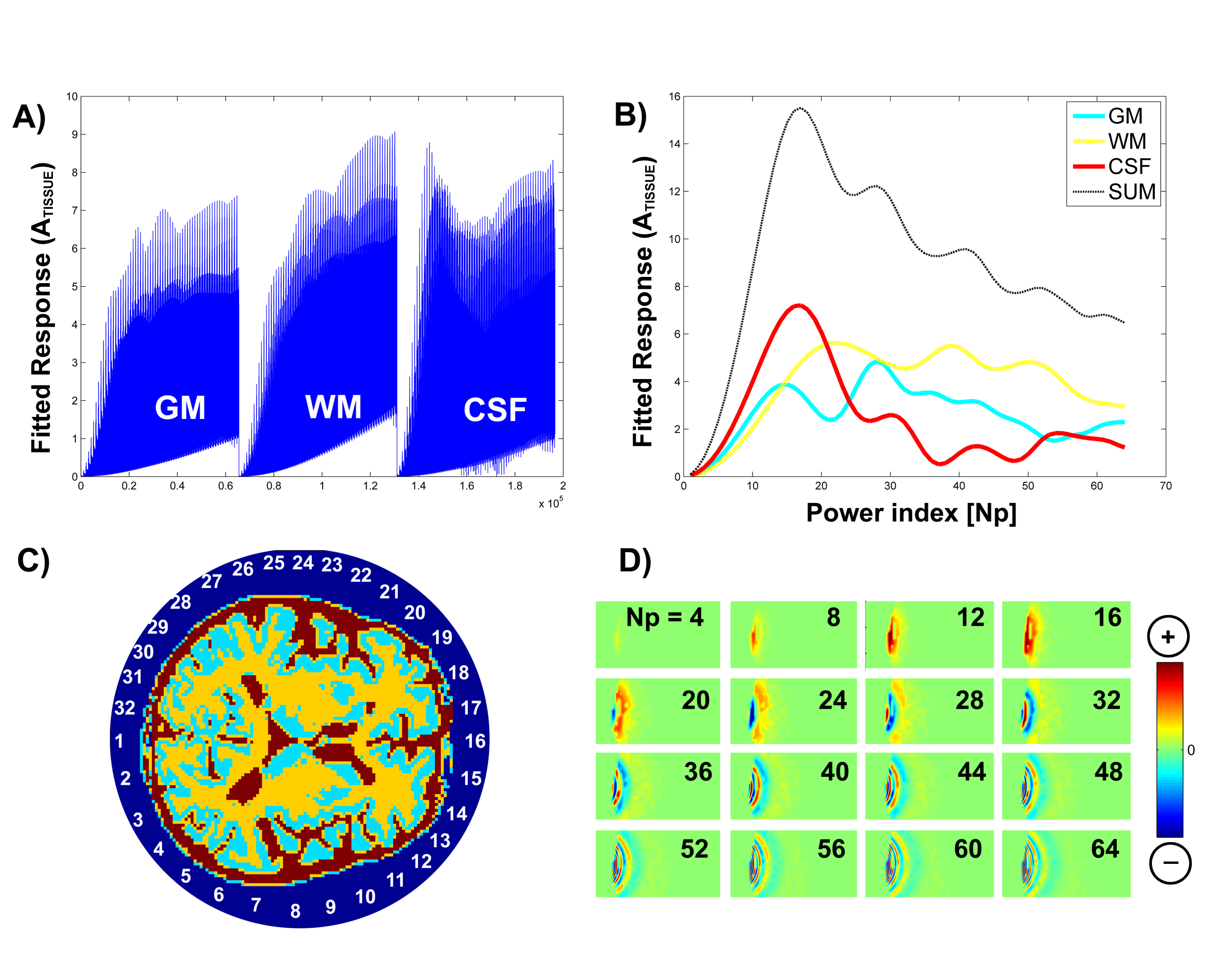
Previous work in silent MRI1 has shown that a homogeneous transmit with linearly varying B1 phase can be used to traverse k-space. Analogously, linearly varying B1 magnitude fields can achieve a similar result. Spatial encoding can be achieved using a surface coil’s spatial B1 amplitude profile to create a relationship between transmit power and duration to the flip angle of the magnetization. The result is a transverse magnetization with banding artifacts (Figure 1D) that act as encoding functions. The issues that arise in reconstruction are primarily due to the non-orthogonality of these encoding functions, prohibiting analytic reconstruction. It can be shown that particular subsets of power levels can be chosen to increase orthogonality between transmitters and receiver pairs. Unfortunately, this subset quickly exceeds SAR limitations and can vary between receivers. As such, it would be beneficial to create a reconstruction method that can use signal modulation due to small changes of power for image reconstruction. Here we show this can be achieved using deep machine learning for reconstruction.
Methods
Neuroimaging data used to generate simulated signals were obtained from the Alzheimer’s Disease Neuroimaging Initiative (ADNI) database (adni.loni.usc.edu). The first 1100 images from this database meeting the following criteria were selected: a static field strength of 3 Tesla, axial orientation, 1 mm isotropic, with T1 weighting. Matlab (the Mathworks, INC. Natick, MA) was used in conjunction with SPM8 (Statistical Parametric Mapping2) to decompose each image into the three tissue classes: GM, WM, and CSF. Two separate pulse sequences were examined, i) a long TR between pulses such that a FID can be measured to extract tissue components as shown in Figure 1B, and ii) where one data point is acquired (~1us) in intervals during the transmit pulse such that the recorded signal is the proton density weighted sum shown in Figure 1 B). A 32 channel RF coil was used as shown in Figure 1 C. Each RF coil was circular and evenly spaced around a 30 cm diameter former with 10% overlap for decoupling purposes3. Transmit and receive B1 fields from each RF coil were calculated ignoring wavelength effects. Independent transmit and receive B1 profiles were achieved with low impedance amplifiers4. The power applied to each transmit element was increased in a quadratic manner resulting in power increase from 0 to 36dB. A constant scale factor was introduced to yield a reasonable power curve, approximately within safety limitations as shown in Figure 1B. A 2D approach for reconstruction employed a constant gradient in the z direction to allow simultaneous multi-slice imaging5. From the 1100 3D images, only 21,600 axial 2D images with a mean signal above a threshold were included in the final data set. The simulated signals for each combination of 32 transmit elements, 32 receiver elements, and 64 transmit powers forming a tensor was used as input into the deep machine learning neural networks6.Results and Discussion
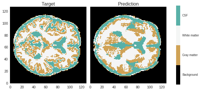
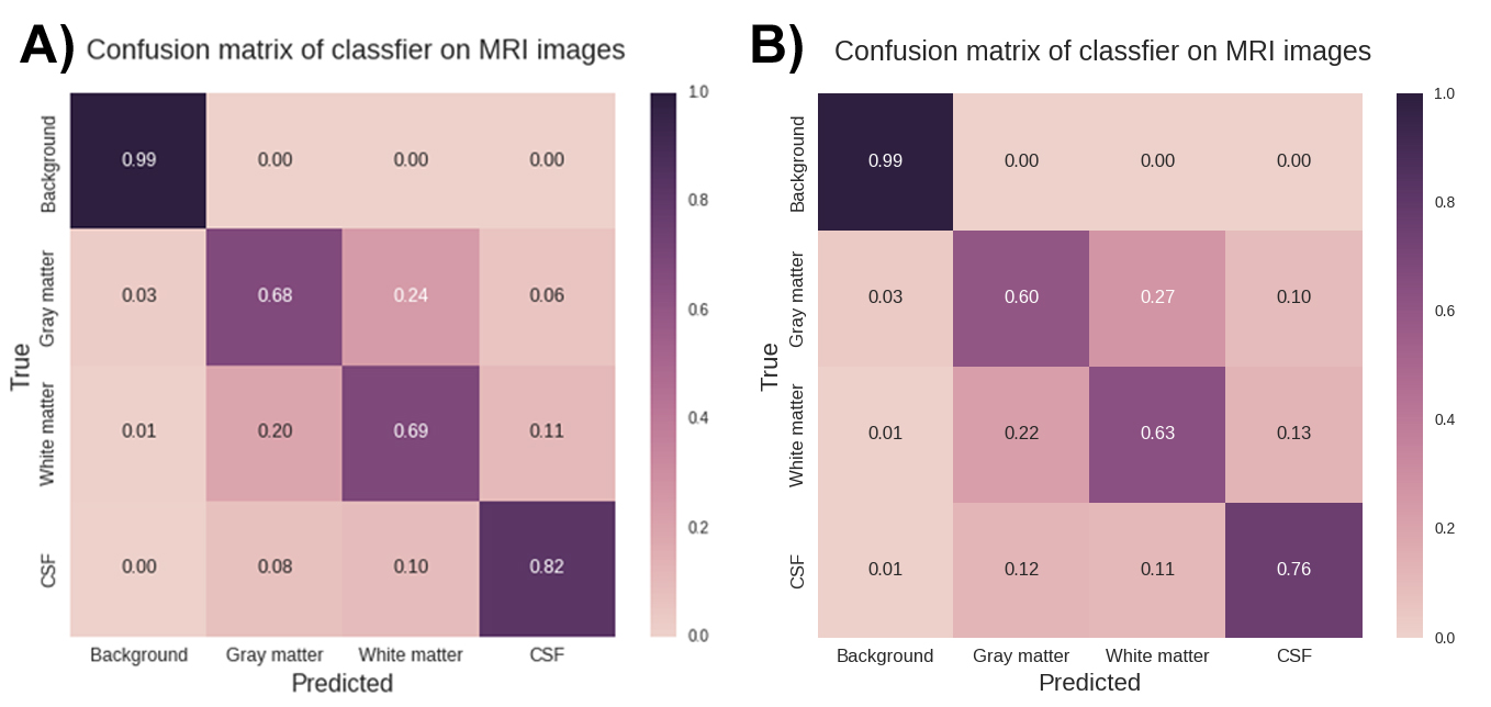
A representative image reconstruction is shown in Figure 2. The encoding of higher spatial frequencies in the periphery do not translate to higher classification accuracy. The high anatomical variations in cortical folding patterns appears to drive the miss-classification, whereas deep brain CSF appears to have higher classification accuracy than expected. The confusion matrix from each method is shown in Figure 3. The decrease in classification accuracy for the proton density data is a minor setback compared to the gain of 2-3 orders of magnitude on the temporal efficiency.
Current assumptions that were used in this study, but which require further investigation include wavelength effects for improved B1 estimation and safety limits, and the introduction of noise. The addition of more subjects in the training set would also improve the classification of cortical structures known to have a high degree of anatomical variation.
Acknowledgements
We thank Yuzo Kanomata for computing support, and Daniel Whiteson for useful discussions. We acknowledge support from the National Science Foundation (Grant No. IIS-1550705 to PB and Graduate Research Fellowship Grant No. DGE 1106400 to C. E.). We are also grateful to NVIDIA for a hardware grant to PB.References
[1] J. C. Sharp and S. B. King, “MRI using radiofrequency magnetic field phase gradients,” Magnetic Resonance in Medicine, vol. 63, no. 1, pp. 151–161, 2010. [2] Ashburner, J. & Friston, K. Multimodal image coregistration and partitioning--a unified framework. NeuroImage 6, 209–217 (1997). [3] Roemer, P. B., Edelstein, W. A., Hayes, C. E., Souza, S. P. & Mueller, O. M. The NMR phased array. Magn. Reson. Med. 16, 192–225 (1990). [4] Chu, X., Yang, X., Liu, Y., Sabate, J. & Zhu, Y. Ultra-low Output Impedance RF Power Amplifier for Parallel Excitation. Magn. Reson. Med. 61, 952–961 (2009). [5] Weaver, J. B. Simultaneous multislice acquisition of MR images. Magn. Reson. Med. 8, 275–284 (1988). [6] He, K., Zhang, X., Ren, S. & Sun, J. Delving Deep into Rectifiers: Surpassing Human-Level Performance on ImageNet Classification. ArXiv150201852 Cs (2015).Figures