1471
Quantitative DCE-MRI Accuracy Evaluation Using Dynamic Physical vs. Digital Phantom: a Cross-Validation1Radiology, Mayo Clinic Arizona, Scottsdale, AZ, United States, 2Radiology, Mayo Clinic Arizona, Phoenix, AZ, United States, 3Radiology-Diagnostic, Mayo Clinic, Rochester, MN, United States
Synopsis
To study the image accuracy of quantitative DCE-MRI a digital phantom and computer simulation were usually used. To validate the digital phantom method, we conducted a cross-validation study comparing the image accuracy estimation from simulation with that from a dynamic physical phantom with contrast infusion. Results showed that the estimated errors were usually higher with the physical phantom, likely due to the difference in reproducibility. Consistency was found in the measurement error comparison between imaging techniques when the temporal resolution was high.
Introduction
Quantitative analysis of DCE-MRI are objective measurements of tissue biology and are expected to reduce variability across institutions and scanner platforms. For that purpose, significant efforts have been made and are still needed in evaluating the accuracy of these quantitative techniques [1-4]. The impact of accelerated imaging techniques on quantitative measures were usually evaluated using a digital phantom and computer simulation [3-6]. However, true validation is challenging partially due to the lack of gold standard physical dynamic phantom available which can accurately and reliably reproduce the contrast kinetics. In this study we compared results using a dynamic digital with a physical phantom as a cross-validation.Methods
A 3T clinic scanner (Skyra, Siemens Healthcare) and TWIST sequence [5] were used in this study. The simulation method was described in detail in [3, 4]. As shown in Figure 1, each k-space view was multiplied with enhancement at that time point based on the view order from the raw data or protocol file. The modified k-space data were written back to the raw data file and reconstructed using Siemens image reconstruction pipeline. A home-made flow resistive cylindrical phantom shown in Figure 2 was used in this study. This phantom has a diameter of 4 cm and length 9 cm, and was filled with polyester fiber. Five scans were performed: (1) 8 slices 3D spoiled gradient echo with temporal resolution of 1.52 s per frame (called “fast scan”) and fully sampled; (2) 52-slices spoiled gradient echo with 10 s per frame and fully sampled (‘Full’); (3) repeat (1); (4) 52 slices spoiled gradient echo with TWIST under-sampling (A=10%, B=25%), 3 s per frame (‘TWIST’); and (5) repeat (1). All parameters were kept the same except slice number. The physical phantom was first ‘perfused’ with deionized water for 1 minute before each scan and was continuously perfused until the end of the scan. For each scan 2 ml Contrast (Gadovist) was infused into the phantom after first time frame or about 10 seconds, the injection rate= 2ml/s. FOV = 120 mm and slice thickness = 5 mm. Matrix 64 x 64. TR=4ms, TE=1.55ms, flip angle=9o. Simulated Full and TWIST raw data were generated using the simulation method shown in Figure 1. The digital phantom was generated by masking the enhanced area in scan (3). Because scan (3) was acquired between ‘Full’ and ‘TWIST’, system drift was minimized, therefore scan (3) was considered as the ‘Ground truth’ enhancement. To generate simulated ‘Full’ and ‘TWIST’ we replaced the k-space data from the acquired raw data file of ‘Full’ and ‘TWIST’ with the simulated data. All images were reconstructed from the simulation system. The RMS error for the whole curve (RMSall) and at the peak contrast (RMSpeak) [3], as well and the Ktrans and ve with Tofts model, were calculated for both acquired and simulated images.Results
Figure 3a shows the enhancement from (1), (3), and (5) as reasonably reproducible. Figure 3b and 3c demonstrated that the average enhancement from simulated ‘Full’ and ‘TWIST’ were both very close to the ‘Ground Truth’, while the enhancement from acquired data were reasonably close. The RMS errors and PK parameters estimated from these images are listed in Table 1. RMS errors were consistently lower for Full than TWIST except RMSpeak for simulated data, which may be due to the high variability caused by the low temporal resolution. For PK modelling (Figure 4), the Ground Truth were: Ktrans=4.4min-1 and ve=0.85. TWIST (acquired or simulated) consistently under-estimate the PK parameters. In Full data sets the results were not so consistent, probably because the tRes was too low for PK analysis.Discussions and Conclusions
This cross-validation study demonstrated that the estimated measurement errors were usually higher with the physical phantom compared to the digital phantom, which is likely due to the difference in reproducibility between the two types of phantoms. Consistency was found in the measurement error comparison between imaging techniques when the temporal resolution was high enough. With Tofts model for this phantom Ktrans was flow limited whle ve theoretically should be 1 as there was no ‘intracellular’ space. Future studies may include multiple acquisitions for variability testing and testing with an intravascular contrast modelling.Acknowledgements
We would like to thank the technologists for their help with the experiment set up.References
1. Sullivan, D., The Quantitative Imaging Biomarkers Aliance (QIBA). Proc. Intl. Soc. Mag. Reson. Med, 2016. 24: p. 6875.
2. Jackson, E.F., Reproducibility & Standardisation of MR Biomarkers, in Proc. Intl. Soc. Mag. Reson. Med. . 2016: Singapore. p. 6876.
3. Le, Y., et al., Evaluation of the Errors in the Measured Dynamic Contrast Enhancement with TWIST View Sharing Using a Novel Simulation Strategy, in ISMRM. 2015: Toronto. p. 4897.
4. Le, Y., et al., A Prototype Image Quality Assurance System for Accelerated Quantitative Breast DCE-MRI, in ISMRM. 2016: Singapore. p. 1271.
5. Song, T., et al., Optimal k-space sampling for dynamic contrast-enhanced MRI with an application to MR renography. Magn Reson Med, 2009. 61(5): p. 1242-8.
6. Bauman, G., et al., Three-dimensional pulmonary perfusion MRI with radial ultrashort echo time and spatial-temporal constrained reconstruction. Magn Reson Med, 2015. 73(2): p. 555-64.
Figures
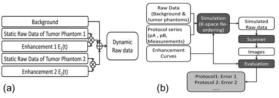
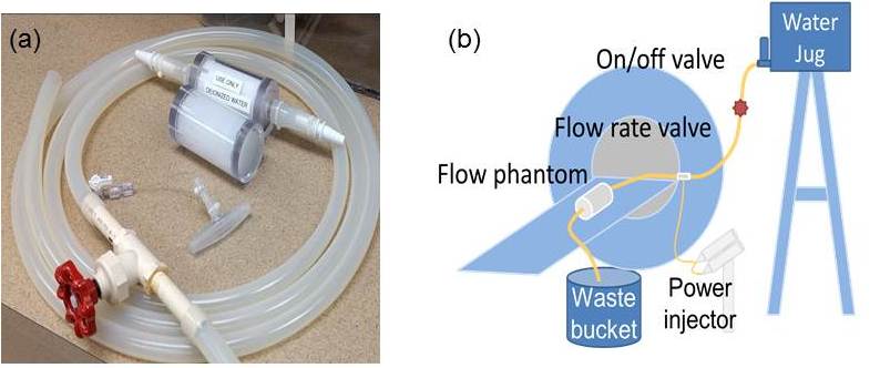
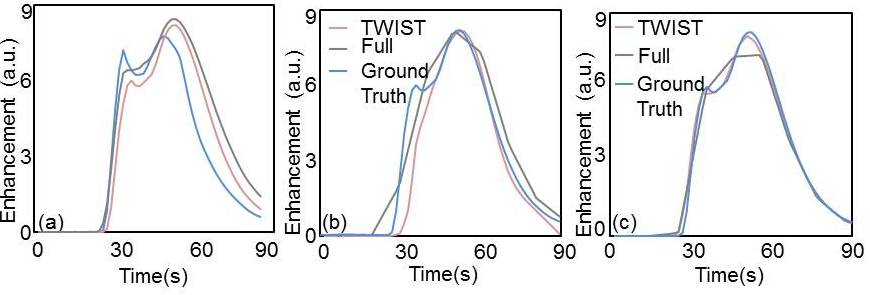
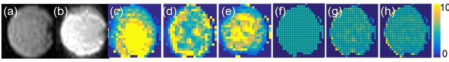
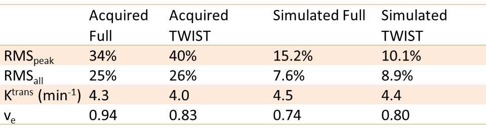
Table 1: Measurement Accuracy in acquired and simulated DCE-MRI