Methods

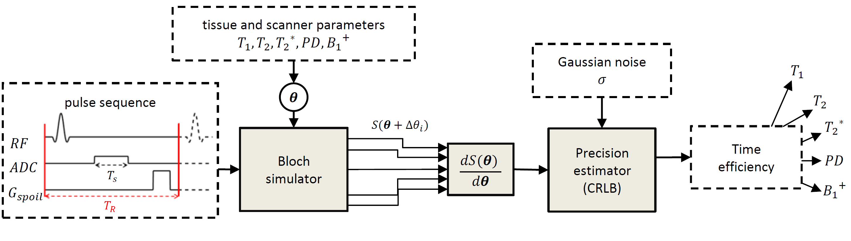
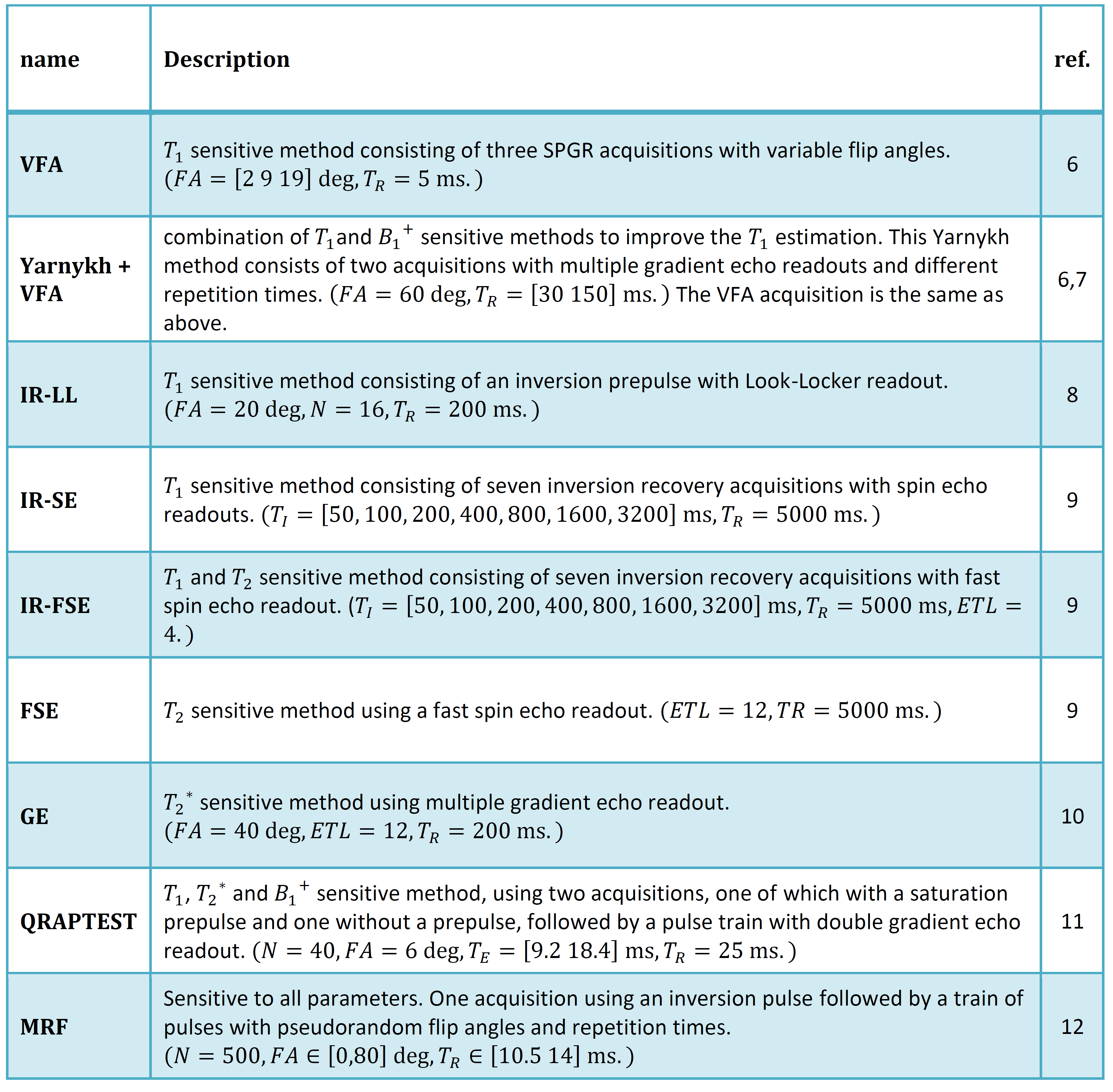
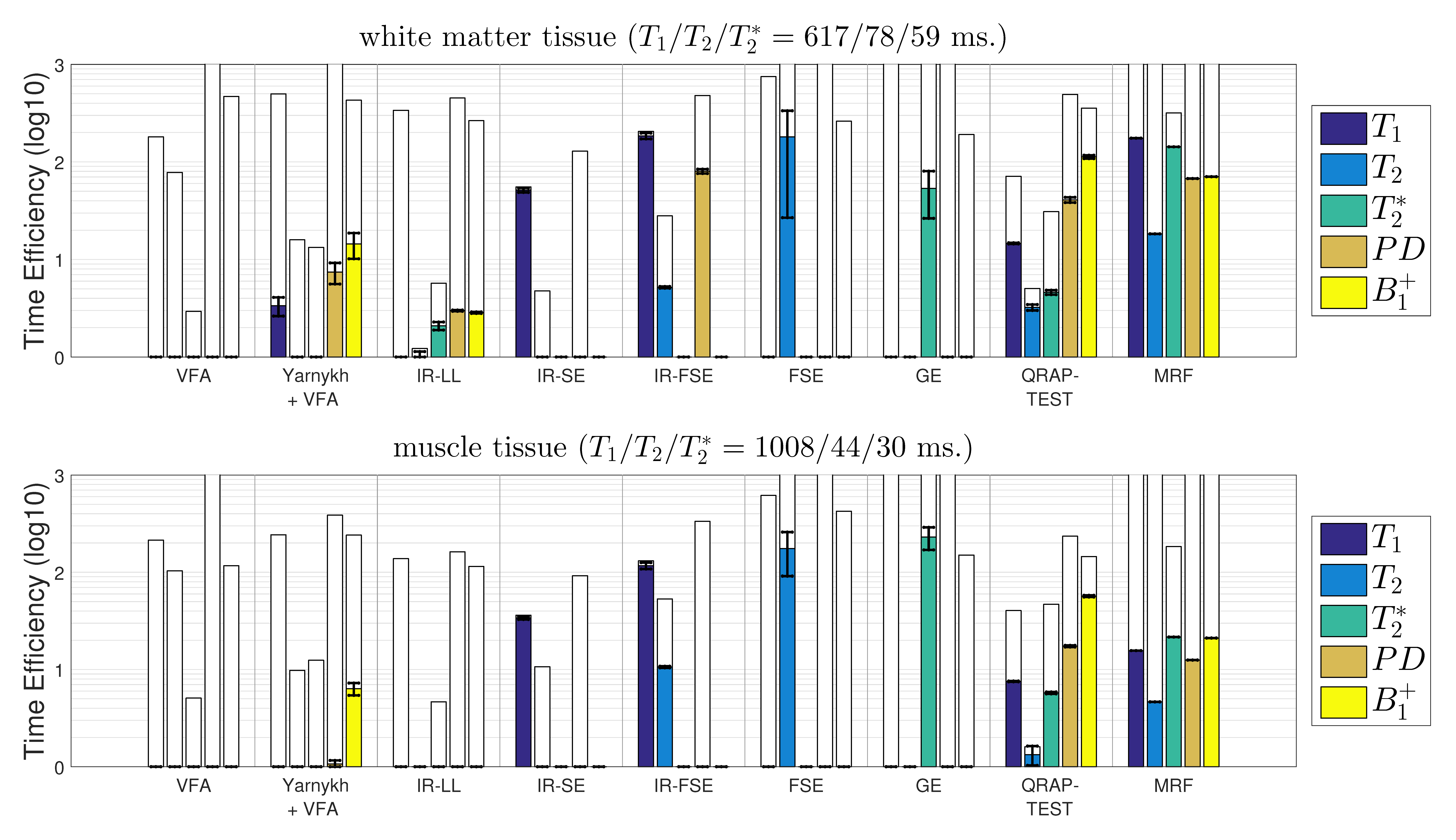
Quantitative MRI (qMRI) methods conventionally measure the proton density, $$$PD$$$, spin-lattice relaxation time, $$$T_1$$$, spin-spin relaxation time, $$$T_2$$$, and the apparent spin-spin relaxation time, $$$T_2^*$$$. This often requires knowledge of the (local) radiofrequency transmit field scaling, $$$B_1^+$$$. For a given qMRI pulse sequence and parameters $$$\theta:=(T_1, T_2, T_2^*, PD, B_1^+)$$$, the Bloch equations describe the expected MRI signal, $$$S(\theta)$$$. The information that $$$S(\theta)$$$ contains on the underlying parameters can be expressed by the Fisher matrix ¹: $$\mathcal{I}(\theta) = \frac{1}{\sigma^2} \left(\frac{\partial S(\theta)}{\partial \theta}\right)^T \left(\frac{\partial S(\theta)}{\partial \theta }\right) \in \mathbb{R}^{5\times 5}, $$ where $$$\sigma $$$ equals the noise level. The Cramér-Rao lower bound (CRLB) theorem states that $$$\Sigma(\theta ):=\mathcal{I}(\theta )^{-1}$$$ is a lower bound on the covariance matrix of any unbiased estimator of $$$ \theta$$$ ¹. We assume that for each qMRI sequence, we can construct such an unbiased estimator of $$$\theta$$$ that attains the CRLB, for instance by using a maximum likelihood estimator ^2,3. Accordingly, we define the precision with which a parameter $$$\theta_i$$$ can be estimated by $$$\Sigma_{i,i}(\theta )^{-1}$$$. The upper limit of the precision is given by $$$\mathcal{I}_{i,i}(\theta)$$$. However, this bound is only reached when the signal response to a change in $$$\theta_i$$$ is not correlated to changes induced by the other MR parameters. The precision is normalized to compensate for differences in tissue parameters and scan time: $$\bar{\mathcal{I}}(\theta):=D^T\mathcal{I}(\theta)D/T_{acq} + P \in \mathbb{R}^{5\times 5},$$ where $$$T_{acq}$$$ equals the scan time, and $$$D$$$ and $$$P$$$ are diagonal matrices that respectively contain reference values of $$$\theta$$$ and a small amount of prior knowledge to ensure $$$\bar{\mathcal{I}}(\theta)$$$ is invertible. We define the time efficiency with which a parameter can be estimated as $$$\theta_i$$$ as $$\mathcal{E}_i(\theta) := \left(\bar{\Sigma}_{i,i}(\theta)\right)^{-1} \in \mathbb{R}.$$ $$$S(\theta)$$$ was obtained with Bloch simulation ⁴ for a variety of qMRI methods, each modeled as ordered sequences of RF pulses, gradient waveforms, readout time, and delays, see Table 1. Both the RF and gradient pulses were modeled as instantaneous effects. In order to simulate $$$T_2’$$$ decay, the signal was based on an ensemble of spins with a Cauchy distribution of off-resonance frequencies ⁵. The k-space sampling strategy was not modelled as our time efficiency measure is invariant to the chosen k-space trajectory. Figure 1 shows an overview of our framework. Each sequence was simulated for white matter ($$$T_1/T_2/T_2^* = 617/78/59$$$ ms) and muscle tissue ($$$T_1/T_2/T_2* = 1008/44/30$$$ ms), with $$$PD=1000$$$ and $$$B_1^+=1$$$. For each parameter $$$\theta_i$$$, we set $$$D_{i,i}$$$ to the given value, and $$$P_{i,i}=10^{-8}$$$.

Results

Figure 2 shows high time efficiency when qMRI methods estimate the parameters for which they were originally designed. Exceptions were the VFA and IR-LL methods for $$$T_1$$$ estimation. Improved time efficiency can be observed by including $$$B_1^+$$$ measurements in VFA. Generally, the time efficiency of a parameter improved dramatically, when assuming the other parameters are known (compare $$$\bar{\mathcal{I}}_{i,i}(\theta)$$$, white, with $$$\mathcal{E}_i(\theta)$$$, colored). Within the presented selection of methods, maps of multiple parameters are best obtained using QRAPTEST or MRF, while single parameters may be best determined using IR-FSE $$$(T_1)$$$, FSE $$$(T_2)$$$, or GE $$$(T_2^*)$$$. Time efficiency values show a small decrease when moving from white matter to muscle tissue which has a lower expected SNR.

Discussion

The results demonstrate that our framework is applicable to a range of qMRI sequences and tissues. Furthermore, the derived time efficiency measure is useful for sequence comparison. Clearly, some methods (e.g. VFA) cannot provide precise estimation without knowledge on the other parameters ($$$B_1^+$$$). A limitation of our work is that by normalizing with the time duration, differences in the minimally scan time required in practice are not considered. Furthermore, we do not model factors such as subject movement and blood flow. Therefore, future research will evaluate if the differences in time efficiency match actual time efficiency differences in the scanner. In this work we show a selection of methods in order to introduce our time efficiency measure. However, the proposed framework can test any qMRI sequences and settings in sillico, without requiring a costly scanner implementation.

Conclusion

Our framework for determining the time efficiency of quantitative MRI sequences is applicable over a wide range of sequences, settings, and tissue types. As such, it is a versatile, practical tool for designing qMRI experiments and theoretical insight into MR sequences.

Acknowledgements

No acknowledgement found.