1450
Regional variations in cerebral venous contrast using susceptibility-based MRI1Monash Biomedical Imaging, Monash University, Clayton, Australia, 2Faculty of Information Technology, Monash University, Clayton, Australia, 3Monash Imaging, Monash Health, Clayton, Australia, 4The Australian eHealth Research Centre, CSIRO Health and Biosecurity, Australia, 5Department of Anatomy and Neuroscience, The University of Melbourne, Melbourne, Australia, 6Monash Immersive Visualisation Platform, Monash University, Clayton, Australia, 7ARC Centre of Excellence for Integrative Brain Function, Melbourne, Australia
Synopsis
In this study we compared the image contrast properties of susceptibility-weighted imaging (SWI) and quantitative susceptibility mapping (QSM) for cerebral venous identification and visualisation. SWI and QSM are minimally invasive techniques to image cerebral veins with distinct contrast properties. We hypothesised that these techniques would provide complementary vein contrast in different brain regions. Contrast was measured using 1072 manually traced vein images from ten volunteers. We found regional variations in the predictive power of vein contrast and computed maps of contrast profiles that may inform which technique is best for a given application.
Purpose
The paramagnetism of deoxygenated haemoglobin provides an endogenous contrast agent for minimally-invasive MRI imaging of the cerebral veins1. Magnetic susceptibility differences perturb the magnetic field of the MRI, manifesting in the phase component of gradient-recalled echo (GRE) acquisitions. The perturbations due to cylindrical veins are orientation dependent and have varying intravascular and extravascular components. Two techniques designed to exploit this phase information are susceptibility-weighted imaging (SWI)2 and quantitative susceptibility mapping (QSM)3,4. SWI attenuates magnitude signal with high-pass filtered phase information, resulting in improved visibility of small veins by including extravascular contributions. QSM solves the ill-posed field inversion problem using either deconvolution or constrained-regularisation, resulting in an estimate of local magnetic susceptibility.
The distinct vein and non-vein signals expressed in SWI and QSM images may provide complementary vein contrast in different brain regions. In this study we manually traced vein masks, constructed a vein atlas, and computed the predictive power of SWI and QSM voxel intensities to determine where in the brain SWI or QSM contrast were comparatively advantageous for imaging veins.
Methods
Ten healthy volunteers were scanned on a 3T Siemens Skyra with a 32-channel head-neck coil (6 females, mean age 56.2 years, standard deviation 25.2) using a flow-compensated GRE (TE=20ms, TR=30ms, FA=15°; six subjects with voxel=0.9×0.9×1.8mm, matrix=256×232×72; four subjects with voxel=0.9x0.9x0.9mm, matrix=256×232×160). Registration (FNIRT) required a T1-Weighted MPRAGE scan (TE=2ms, TR=2300ms, TI=900ms, voxel=1.0x1.0x1.0mm, matrix=240x256x192, FA=9°). Six subjects were from the ASPREE clinical trial and scanned at baseline in the ASPREE NEURO sub-study5. Raw k-space was retrospectively reconstructed per channel. QSM was computed using Laplacian unwrapping3, V-SHARP4 background field removal and LSQR (STI-Suite3). SWI images were taken from the scanner console.
Vein contrast was assessed using manually traced ground-truth vein masks ($$$Y$$$) by comparing the predictive power of normalized image intensities ($$$\dot{X}_i$$$, where $$$i\in\{SWI,QSM\}$$$). A map of predictive power for an image, $$$P_i(\dot{X}_i,Y)$$$, was calculated using log-loss6.
$$P_i(\dot{X}_i,Y)=-log(Y⋅(1-\dot{X}_i )+(1-Y)⋅\dot{X}_i)$$
Cohort mean $$$P_i$$$ maps was constructed from co-registered subject maps and compared.
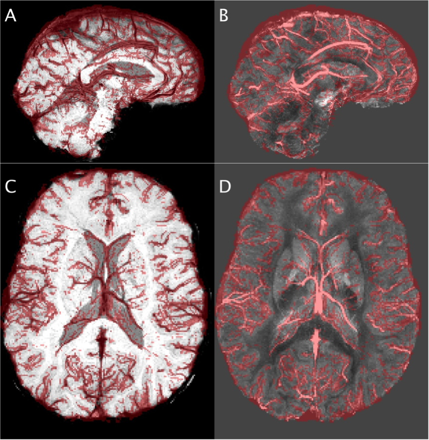
Vein masks were manually traced (FSLView) by an author under a clinical radiologist’s supervision using both SWI and QSM images (e.g. Figure 1). Vein voxels were given a 0.9 score and non-vein voxels 0.1, i.e., $$$Y\in\{0.9=V,0.1=N\}$$$, to reflect human mutability.
The normalization process did not use the manual tracings. QSM intensities, $$$X_{QSM}$$$, were normalized, $$$\dot{X}_{QSM}$$$, using an unsupervised Gaussian Mixture Model (GMM) (initial labels QSM>0.05ppm). The GMM parameters were fit using expectation-maximization. The same process was applied to SWI, using the same initial labels.
$$\dot{X}_i=\frac{Pr(X_i=V,\Omega_i)}{Pr(X_i=V,\Omega_i)+Pr(X_i=N,\Omega_i)}$$
where $$$\dot{X}_i$$$ is the normalized contrast, $$$Pr(X_i=x,\Omega_i)$$$ is the likelihood of $$$X_i$$$ having label $$$x\in\{Vein=V,Non-Vein=N\}$$$ given GMM parameters $$$\Omega_i=\{\mu_{i,V},\mu_{i,N},\sigma_{i,V},\sigma_{i,N},\omega_{i,V},\omega_{i,N}\}$$$ (mean, variance and mixture weight respectively).
A vein atlas, $$$\dot{X}_{Atlas}$$$, was constructed for each subject by taking the mean of vein tracings from all other subjects (to ensure independence) and co-registering them to the subject’s space. A third map, $$$P_{Atlas}$$$, was calculated for $$$\dot{X}_{Atlas}$$$.
Results
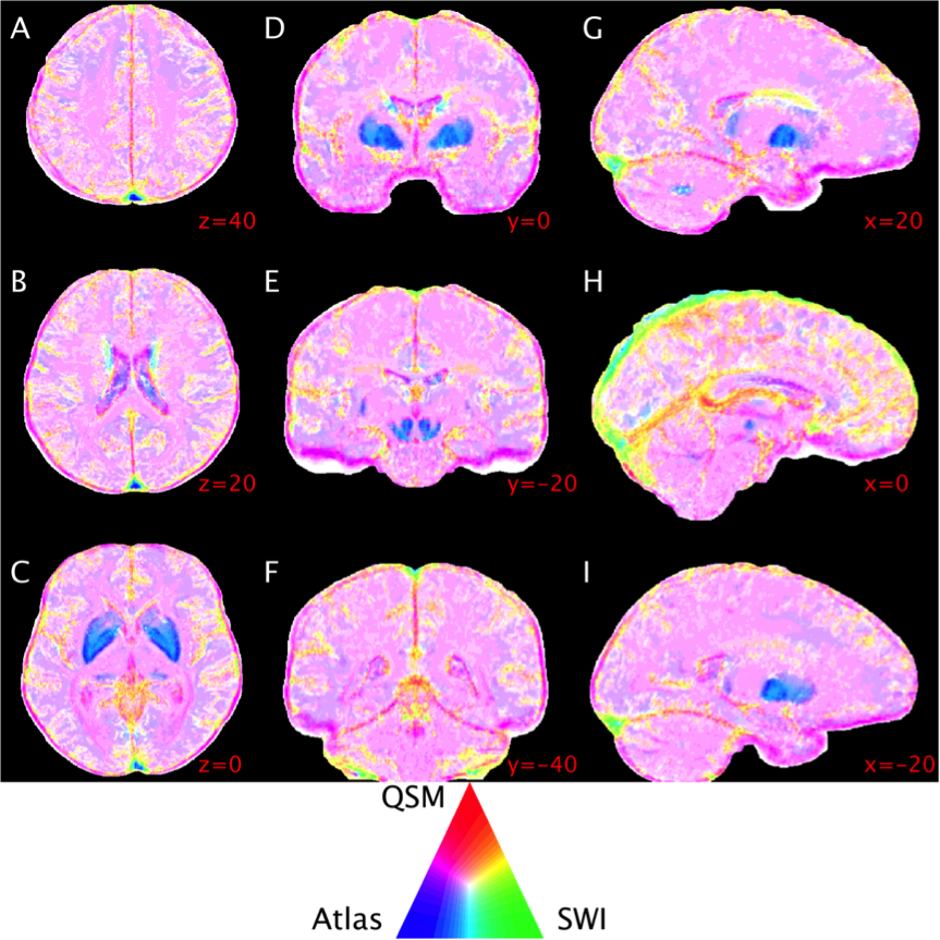
Predictive power throughout the brain was highly heterogeneous, particularly near large venous sinuses, iron-accumulating deep-grey matter structures and in interstitial spaces (Figure 2). QSM had comparatively higher power near low-signal structures, e.g. falx cerebri, and lower power in the deep-gray matter structures, relative to SWI and the atlas. The atlas was highest in the deep-gray matter, particularly on structure boundaries. SWI had higher predictive power on the superior surface of the cortex and near large venous sinuses, and lower power on the inferior surface of the brain. The majority of the brain tissue was best represented by a combination of QSM and the atlas (pink hue in Figure 2).Discussion and Conclusion
Larger veins on the surface of the brain, e.g. superior sagittal sinus, were best depicted by SWI and the atlas, possibly due to phase processing artefacts in QSM images. SWI appeared to be confounded by low magnitude-signal structures, e.g. falx cerebri and tentorium. Iron accumulation in the deep-grey matter structures appears to confound both QSM and SWI, with highest relative power coming from the atlas. However, the predictive power of the atlas was also low, due to anatomical variation. The higher predictive power of the SWI in the centre of these structures may be a result of high-pass filtering.
Future work will include: investigation of the sensitivity of QSM results to acquisition and processing methods; and, development of an image post-processing technique to combine SWI, QSM and an atlas into a single vein image.
In summary, using manually traced vein masks we have computed the variation in SWI and QSM vein contrast across different brain regions and determined where the SWI and QSM techniques were comparatively advantageous for imaging veins.
Acknowledgements
We thank the investigators of the ASPREE study and the ASPREE-NEURO sub-study for the coordination and recruitment of the volunteers. We thank the volunteers for their time and willingness to participate.
The Alzheimer’s Australia Dementia Research Foundation (AADRF), the Victorian Life Sciences Computation Initiative (VLSCI), the Multi-model Australian ScienceS Imaging and Visualisation Environment (MASSIVE) and the National Health and Medical Research Council (NHMRC) supported this work (NHMRC Grant APP1086188).
References
1. Reichenbach JR, Venkatesan R, Schillinger D, Kido D, Haacke E. Small vessels in the human brain: MR venography with deoxyhemoglobin as an intrinsic contrast agent. Radiology. 1997;204(1):272–277.
2. Haacke EM, Xu Y, Cheng Y-CN, Reichenbach JR. Susceptibility weighted imaging (SWI). Magn Reson Med. 2004;52(3):612-618. doi:10.1002/mrm.20198.
3. Li W, Avram AV, Wu B, Xiao X, Liu C. Integrated Laplacian-based phase unwrapping and background phase removal for quantitative susceptibility mapping. NMR Biomed. 2014;27(2):219-227. doi:10.1002/nbm.3056.
4. Wu B, Li W, Guidon A, Liu C. Whole brain susceptibility mapping using compressed sensing. Magn Reson Med. 2012;67(1):137-147. doi:10.1002/mrm.23000.
5. Ward SA, Raniga P, Ferris NJ, et al. ASPREE-NEURO study protocol: A randomized controlled trial to determine the effect of low-dose aspirin on cerebral microbleeds, white matter hyperintensities, cognition, and stroke in the healthy elderly. Int J Stroke. September 2016:1747493016669848. doi:10.1177/1747493016669848.
6. Good IJ. Rational Decisions. J R Stat Soc Ser B Methodol. 1952;14(1):107-114.
Figures