Synopsis

Double-echo in steady-state (DESS) is a 3D sequence which offers both morphological images and quantitative parameter maps (SNR-efficient 3D maps of T2 and apparent diffusion coefficient (ADC)) in various applications, such as breast imaging or knee cartilage imaging. The sequence has less sensitivity to ADC than to T2, sometimes leading to noisy ADC maps. Here, we investigate the effects of using regularized fitting of the signals, with a penalty in ADC variability, to produce less noisy ADC maps. The method is designed to apply less regularization to regions with high SNR. The approach makes use of a recent analytical expression for a ratio between DESS signals.

Purpose

Methods

The DESS sequence produces signals S₁ before and S₂ after a spoiler gradient^1,2,3. For estimating ADC, DESS is run twice, with a large and small spoiler gradient. This gives high and low diffusion sensitivity for the two scans, labeled H and L, respectively, producing four signals S_1H, S_2H, S_1L, and S_2L. It has been shown that the ratio f=(S_2HS_1L/S_1HS_2L) is sensitive to ADC while being insensitive to T₁ and T₂⁴. This, combined with a variation of a recently developed expression for f⁵, allows a simple regularization that penalizes rapid change in ADC and produces less noisy ADC maps:

$$ \min_{\Delta ADC} \left\lVert \frac{S_{2H}S_{1L}}{S_{1H}S_{2L}} - f(ADC + \Delta ADC)\right\lVert^2 + \lambda \left\lVert D_{xy}(ADC + \Delta ADC) \right\lVert^2 \hspace{5cm}[1]$$

where D_xy is a difference operator between neighboring pixels. By multiplying the left-hand side with S_1HS_2L, the penalty term matters less for pixels with strong signal, thus making the regularization SNR-weighted:

$$ \min_{\Delta ADC} \left\lVert S_{2H}S_{1L} - S_{1H}S_{2L} f(ADC + \Delta ADC)\right\lVert^2 + \lambda \left\lVert D_{xy}(ADC + \Delta ADC) \right\lVert^2 \hspace{5cm}[2]$$

The expression in ref. 5 enables easy linearization of f by doing a first-order Taylor approximation, similar to ref. 6. This turns Eq. 2 into a quadratic equation that is easily solved for a given starting point. This can be iterated until the method converges on a result. This results in fast, regularized estimation.

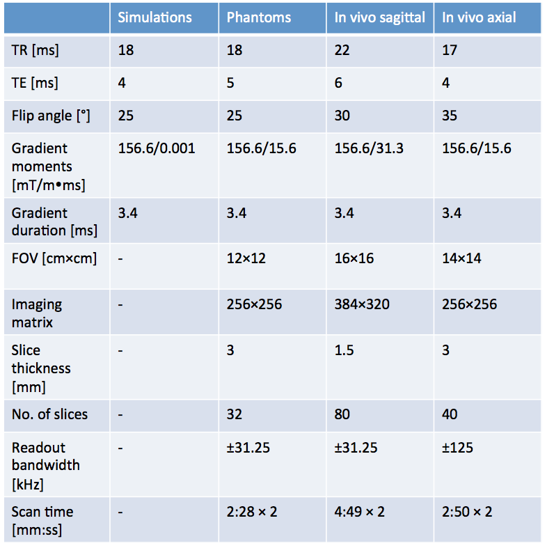
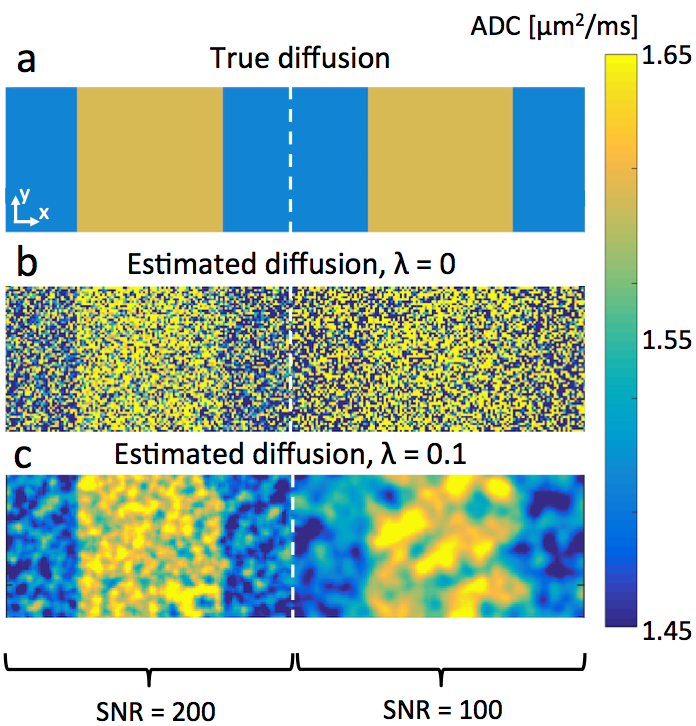
DESS signals were simulated over 256×64 pixels using Extended Phase Graphs (EPG)⁷ (scan parameters in Table 1), with added noise. The tissue parameters were T₁ = 1.2s, T₂ = 40ms, and ADC was made to alternate between 1.6μm²/ms and 1.5μm²/ms, as shown in Fig. 1a. The left half of the image was given twice the signal strength as the right half. This led to an SNR of 100 in the S_1L signal in the right half and 200 in the left half. Eq. 2 was then applied with λ=0 and λ=0.1 (the signals were normalized so that S_1HS_2L=1 on average over the region of interest, or equivalently λ=0.1S_1HS_2L).

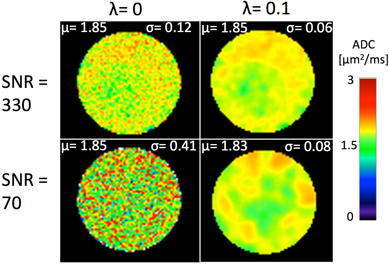
The method was then tested in phantom scans, running two DESS scans with differing diffusion weighting (scan parameters in Table 1). First, a coil giving an SNR of 330 in the S_1L signal was used. Next, the scans were repeated in a coil that gave a lower SNR of 70. ADC was estimated both with λ=0 and λ=0.1. For reference, a standard DWI scan with very low resolution was run.

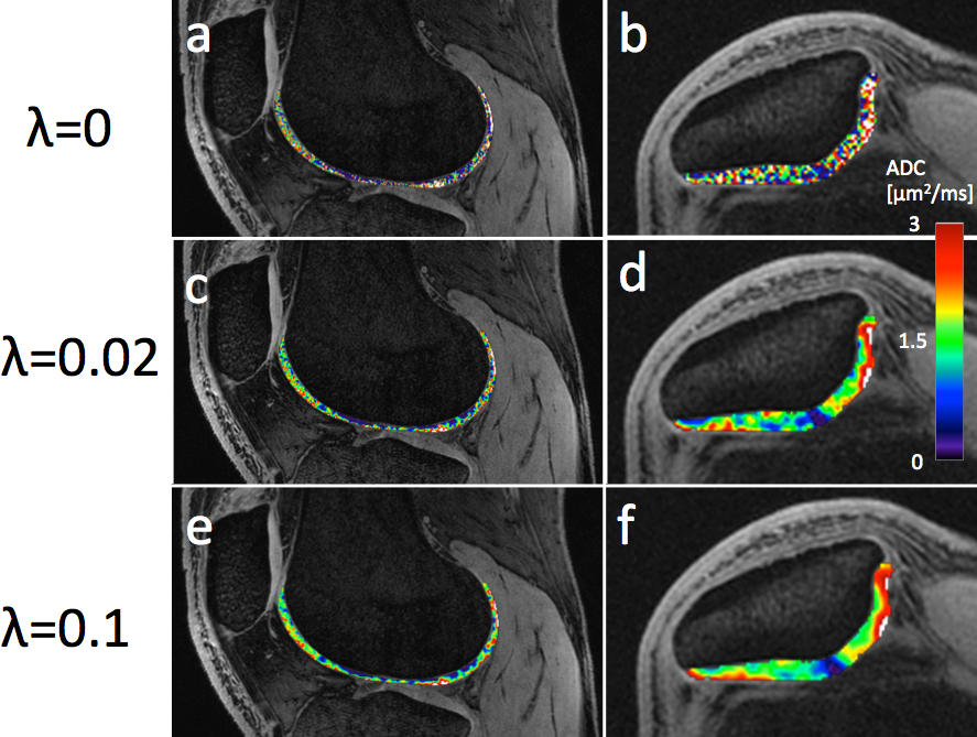
The procedure was then tested in vivo, acquiring a pair of sagittal DESS knee scans in a healthy volunteer and another axial scan pair of another volunteer (parameters in Table 1) and processed with λ=0, 0.02, 0.1.

Results

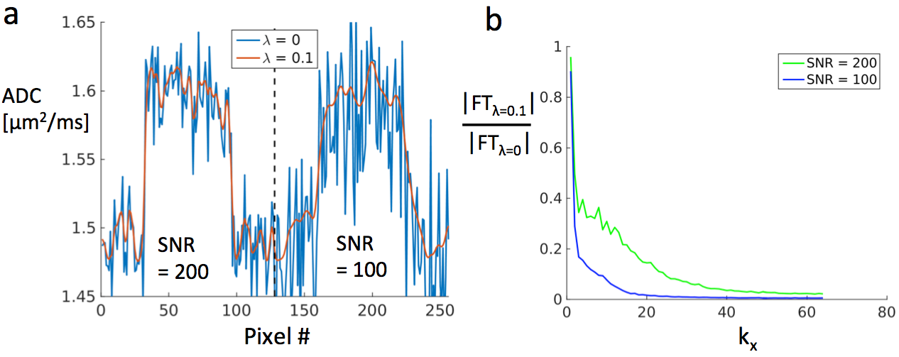
The simulation results are shown in Figs. 1b-c. Fig. 1b, with no regularization, gives noisy estimates, and the structure in the right half (with lower SNR) is hard to discern. Regularized results (Fig. 1c) show the ADC structure more clearly. Since less regularization is applied on the left (having stronger signal), more of the original structure is retained, while the right half is more smoothed. This is also demonstrated in Fig. 2a, which shows the average of each estimate across y. Fig. 2b shows the Fourier transform of the regularized estimate in Fig. 1c divided by that of the unregularized estimate. The regularization clearly suppresses the higher frequency components more as SNR gets lower.

The results from the phantom scans with high SNR showed patterns which were similar after regularization. For the case with low SNR, no particular pattern was discernible without regularization. When regularization was applied, a similar structure as for the high-SNR case became apparent. The estimates are shown in Fig. 3, along with their means and standard deviations, and were all close to the DWI reference value of 2.0 μm²/ms.

The in vivo scans in Fig. 4 show smoother maps with regularization. The regularized maps indicate higher values in superficial cartilage than in deep cartilage, in agreement with ref. 8, which is difficult to discern from the non-smoothed maps (λ=0).

Discussion

Conclusion

Acknowledgements

References