1428
Quantitative Evaluation of Temporal Sparse Regularizers for Compressed Sensing Breast DCE-MRI1School of Science, Nanjing University of Science and Technology, Nanjing, Jiangsu, People's Republic of China, 2Institute of Imaging Science, Vanderbilt University Medical Center, Nashville, TN 37232, 3Institute for Computational and Engineering Sciences, and the Departments of Biomedical Engineering and Internal Medicine, The University of Texas at Austin, Austin, Texas, USA
Synopsis
We quantitatively evaluate temporal sparse regularizers for breast DCE-MRI data under standard compressed sensing schemes. We consider five temporal regularizers on 4.5x retrospectively undersampled Cartesian in vivo breast DCE-MRI data, namely Fourier transform (FT), Haar wavelet transform (WT), total variation (TV), second order total generalized variation (TGV$$$_{\alpha}^{2}$$$) and nuclear norm (NN). Both signal-to-error ratio and concordance correlation coefficients of the derived pharmacokinetic parameters $$$K^{\text{trans}}$$$ (volume transfer constant) and $$$v_\mathrm{e}$$$ (extravascular extracellular volume fraction) are estimated. Results show that NN produces the lowest image error while TV/TGV$$$_{\alpha}^{2}$$$ produce the most accurate pharmacokinetic parameters.
Purpose
Dynamic contrast enhanced magnetic resonance imaging (DCE-MRI) is used in cancer imaging to probe tumor vascular properties$$$^1$$$. Both high temporal and spatial resolutions are beneficial in DCE-MRI; high temporal resolution is needed for quantitative DCE-MRI analysis, while high spatial resolution aids clinical reading. Compressed sensing$$$^2$$$ (CS) theory makes it possible to recover MR images from randomly undersampled k-space data using nonlinear recovery schemes and has been successfully applied to breast DCE-MRI$$$^{3,4}$$$. For dynamic images, since most of the image is roughly constant in time, the most significant redundancy (and hence sparsity) often manifests in the temporal direction. None of these efforts, however, have quantitatively compared different temporal sparsity models for breast DCE-MRI across a large number of sampling patterns. Thus, the purpose of this paper is to quantitatively evaluate common temporal sparsity-promoting regularizers for CS DCE-MRI of the breast.Methods
We considered five ubiquitous temporal regularizers on 4.5x retrospectively undersampled Cartesian in vivo breast DCE-MRI data: Fourier transform (FT), Haar wavelet transform (WT), total variation (TV), second-order total generalized variation (TGV$$$_{\alpha}^{2}$$$), and nuclear norm (NN).
The reconstruction problem solved was $$\hat{X} = \text{arg min}_{X} \frac{1}{2}\left\| AX -B \right\|_{F}^2 + \alpha S(X).$$ Here X is the dynamic image to be reconstructed, $$$A = MF$$$ is the measurement operator, where $$$F$$$ is a spatial Fourier transform on each temporal frame, $$$M$$$ is the sampling mask on each temporal frame, $$$B$$$ is the collected (undersampled) data, $$$\alpha$$$ is a positive, real parameter that balances between data consistency and sparsity, $$$F$$$ is Frobenius norm, and $$$S$$$ is one of the five temporal sparsity-promoting regularizers. We generated 200 distinct Cartesian sampling masks by choosing 200 different random seeds before pattern generation. All the sparse models are solved by the Fast Iterative Shrinkage Thresholding Algorithm$$$^5$$$ for its simplicity and efficiency.
We applied all models retrospectively to in vivo breast DCE-MRI data acquired using a spoiled gradient-recalled echo (SPGRE) sequence on a Philips (Best, Netherlands) Achieva 3T scanner with TR = 4.33 ms, TE = 2.12 ms, flip angle = 12 deg. The dimension of the data was 192 x 192 x 10 x 105, which consisted of 192 readout points by 192 phase encodes across 10 slices repeated over 105 dynamics. To narrow the focus of the abstract, we looked only at the slice that passed through the center of the tumor. For this particular dataset, the center slice was the 6th slice. Also, for all reconstructions, we cropped the image posterior of the chest wall to improve sparsity. The final cropped dimensions of our test data were 192 x 128 in-plane by 105 dynamics.
To evaluate the quality of CS reconstruction, we computed the signal-to-error ratio (SER) of the reconstructed images and estimated concordance correlation coefficients (CCC) of the derived pharmacokinetic parameters $$$K^{\text{trans}}$$$ (volume transfer constant) and $$$v_\mathrm{e}$$$ (extravascular extracellular volume fraction) across a population of random sampling schemes using the Standard Tofts-Kety Model$$$^{6}$$$.
Results
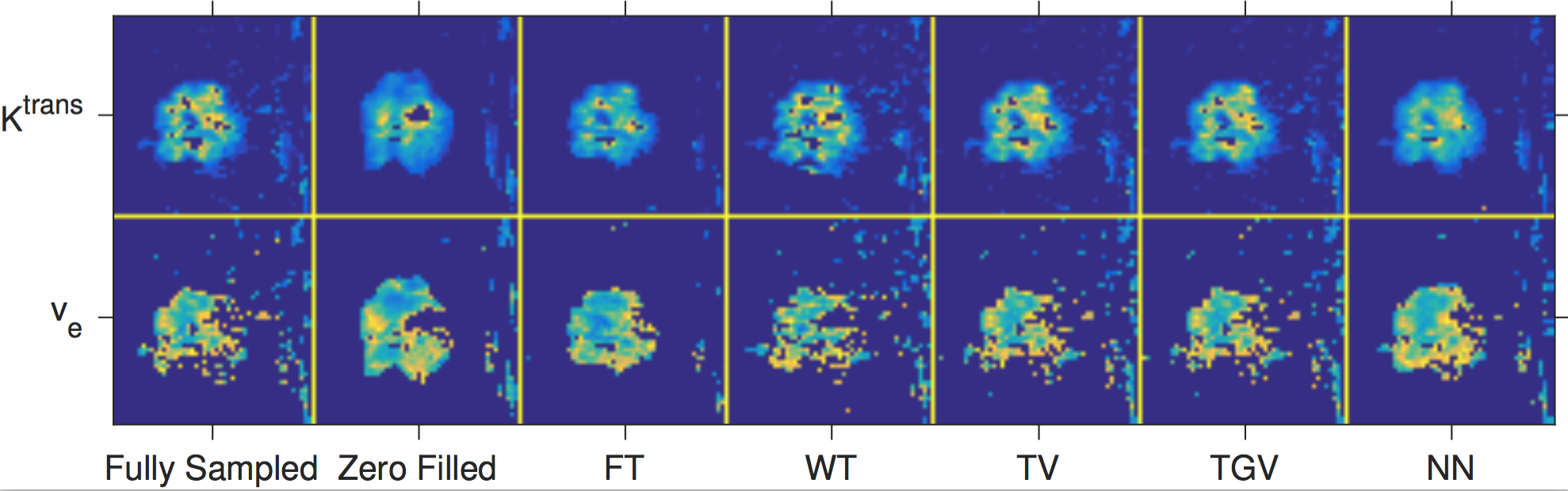
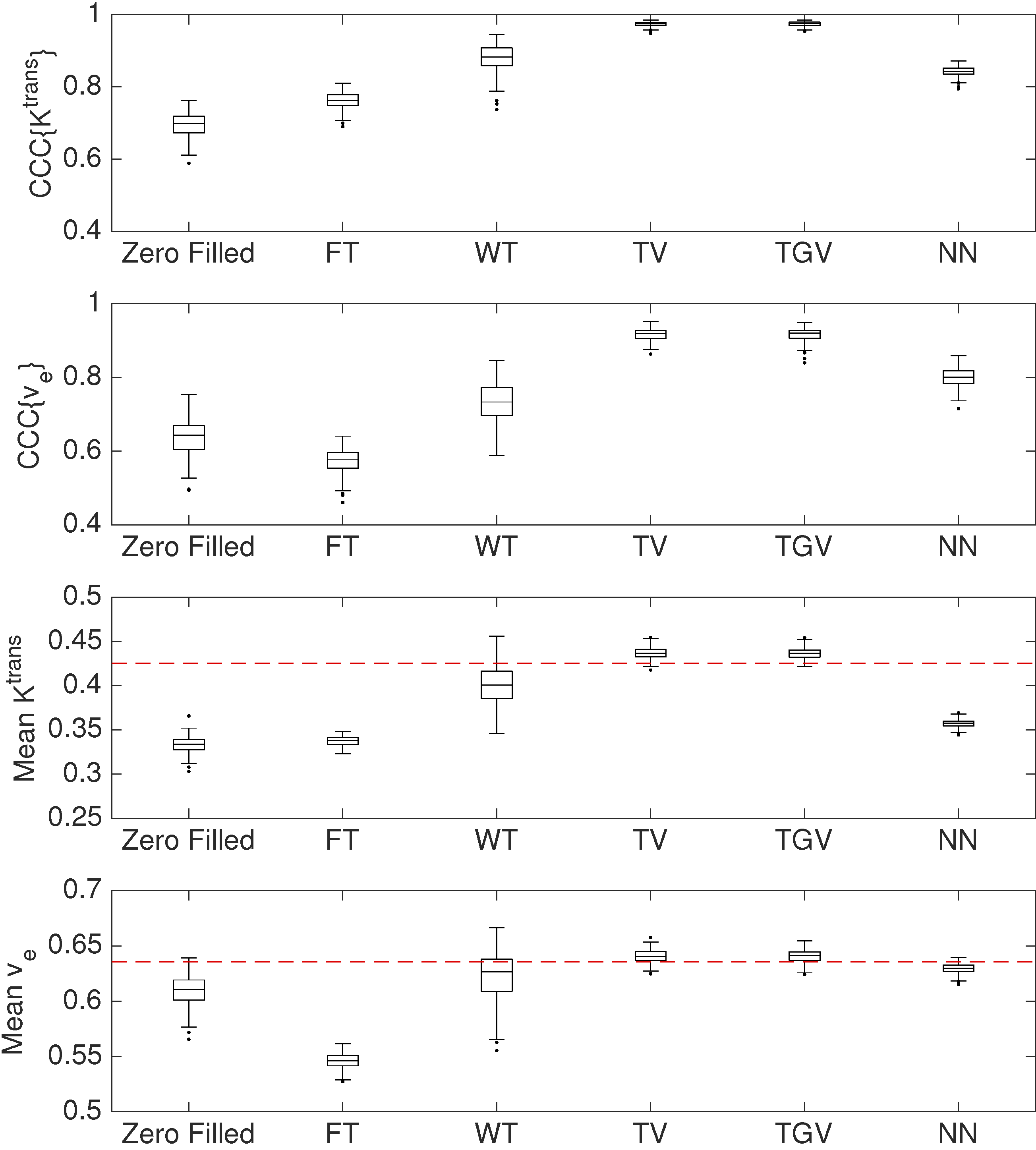
Figure 1 shows zoomed $$$K^\mathrm{trans}$$$ and $$$v_\mathrm{e}$$$ maps of the first sampling pattern. TV, TGV$$$_{\alpha}^{2}$$$, and NN most closely matched the fully sampled tumor.Figure 2 shows the boxplots of CCCs and tumor mean parameters over 200 different sampling patterns. Results show that NN produced the lowest image error (SER: 29.1), while TV/TGV$$$_{\alpha}^{2}$$$ produced the most accurate $$$K^{\text{trans}}$$$ (CCC: 0.974/0.974) and $$$v_\mathrm{e}$$$ (CCC: 0.916/0.917). WT produced the highest image error (SER: 21.8), while FT produced the least accurate $$$K^{\text{trans}}$$$ (CCC: 0.842) and $$$v_\mathrm{e}$$$ (CCC: 0.799).Discussion
The quantitative comparisons showed different performances across the five temporal constraints. TV and TGV$$$_{\alpha}^{2}$$$ provided the best CCCs for $$$K^{\text{trans}}$$$ and $$$v_\mathrm{e}$$$ among the five regularizers tested and also appeared to most closely match the true voxel intensity curves in the tumor area, suggesting that error in fitting the voxel intensity curves may predict the ultimate quantitative parameter accuracy.Conclusions
We compared the quantitative performance of five temporal regularizers for CS DCE-MRI of the breast. The results of the quantitative comparisons presented here should inform clinical and research imaging reconstruction methods. For techniques that value image fidelity above accurate quantitative parameters, the best temporal regularizer may be the nuclear norm. For techniques that value quantitative parameter accuracy above image quality, TV or TGV$$$_{\alpha}^{2}$$$ should be preferred.Acknowledgements
NCI R25 CA092043, NCI K25 CA176219, NSFC 91330101, NSFC 11531005.References
1. Yankeelov TE, Gore JC. Dynamic contrast enhanced magnetic resonance imaging in oncology: theory, data acquisition, analysis, and examples. 2. Lustig M, Donoho D, Pauly JM. Sparse MRI: The application of compressed sensing for rapid MR imaging. Magn Reson Med. 2007. 3. Han S, Paulsen JL, Zhu G, Song Y, Chun S, Cho G, Ackerstaff E, Koutcher JA and Cho H. Temporal/spatial resolution improvement of in vivo DCE-MRI with compessed sensing-optimized FLASH. Magn Reson Imaging. 4. Chen LY, Schabel MC, DiBella EVR. Reconstruction of dynamic contrast enhanced magnetic resonance imaging of the breast with temporal constraints. Magn Reson Imaging. 2010. 5. Smith DS, Li X, Arlinghaus LR, Yankeelov TE, Welch EB. DCEMRI.jl: a fast, validated, open source toolkit for dynamic contrast enhanced MRI analysis. PeerJ 2015. 6. Beck A, Teboulle M. A fast iterative shrinkage-thresholding algorithm for linear inverse problems. SIAM J Imaging Sci 2009.Figures