1427
Flexible convex optimization with non-smooth regularizations for accelerated MRI reconstructions1United-Imaging Healthcare America, Houston, TX, United States, 2Indiana University School of Medicine, Fort Wayne, IN, United States
Synopsis
Convex optimization with non-smooth regularizers has recently gained increased interest as it has shown excellent performance and the ability to facilitate most of reconstruction problems in MR convincible. While there are many approaches towards its fulfillment, a flexible yet easy and comprehensive to realize method is always beneficial. One of the algorithms is proposed in this abstract. and we demonstrate that this algorithm can be easily adapted to many reconstruction problems in MRI with accelerated performance.
Introduction
While there are many approaches
towards fulfillment of convex optimization with non-smooth regularizers, a flexible yet easy and comprehensive to realize
method is always beneficial. One of the
algorithms is proposed in [1], though it’s useful, yet few people ever get
familiar to it. Here, we demonstrate that this algorithm can be easily adapted
to many reconstruction problems in MRI. The original mechanisms and rigorous math
can be retrieved from [1], and an accelerated version combining the idea of
FISTA [2] is presented below. It’s an iterative algorithm which aims at
minimizing a sum of functions by successive evaluations of their gradients or
proximity operators using a proximal algorithm, in which only first-order information of the functions is
exploited. Fenchel–Rockafellar conjugate is involved for proximal operator, which
satisfies the useful Moreau identity. Since the proximity operator of an
indicator function is simply the projection onto the set, proximal algorithms
can be viewed as generalizations of algorithms to find an element in the
intersection of convex sets by successive projections (POCS). The major merits include
ability for high dimensional large-scale optimization, single loop in efficiency,
and simple explicit expressions in coding. Essentially, the method will find $$$x=\arg min_{x}{f(x)+g(x)+\sum_{m=1}^Mh_{m}(L_{m}(x))}$$$,
where the first term can be data consistence in MRI reconstruction,
the second term will be an indicator function, and the multiple (M)
regularizers can be included in the third term. Choose the parameters τ > 0, σ > 0, ρ > 0, t=1 and the initial
estimates x(0), u1(0), …, uM(0),
then iterate, for i = 0, 1, . . ., the optimization can be
performed in the steps of Fig. 1.
Where Lm* is the adjoint operator of
Lm, and $$$pro{x_{\sigma h_m^*}}\left( u \right) = u - \sigma \;pro{x_{h_m^{}/\sigma }}\left( {u/\sigma } \right)$$$Methods
We have used the
above algorithm to GRASP/XDGRASP [3, 4], BCS [5], suppression of MRI truncation
artifact [6], and Single STEP QSM [7] with successes. We will only explain our approach towards GRASP/XDGRASP
and MRI truncation artifact without details on their original concepts. In GRASP/XDGRASP,
regularization of temporal total variations (TVt:= $$${h_m}\left( {{L_m}x} \right)$$$ ) is applied on the
image time series in the reconstruction, Lm and Lm* are temporal
differentiation and its adjoint, and hm and hm* are l1-norm
and its adjoint. proxτg is simply a projection function, and f is the
data consistence in K space. For GRASP m equals 1, and for XDGRASP m equals 2.
The two TVt of XDGRASP work on heart and breath
phase as described in [4]. In
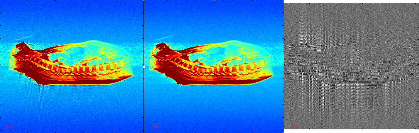
suppression of MRI truncation artifact, regularization of mixture of 1st and
2nd order spatial total variations (TVs:= $$${h_m}\left( {{L_m}x} \right)$$$ ) is applied on the
image in the restoration, Lm=1 and Lm=1* are 1st
order differentiation and its adjoint, Lm=2 and Lm=2* are
2nd order differentiation and its adjoint, and hm and hm*
are l1-norm and its adjoint. proxτg is a projection function, and f is the data consistence in the confidential
region of Fourier domain, the optimization aims to extrapolate the Fourier domain
beyond the confidential region with the later unchanged [6]. For GRASP/XDGRASP, we used the DCE data and
pre-processing code provided by the authors [3, 4] on their website. For
suppression of MRI truncation artifact, we have tested the method on clinical images
acquired with various sequences, as will be demonstrated below.Results
Overall using the current method could earn 3-5 fold acceleration comparing to their original Matlab implementations [3-5, 7]. Without fine tuning of parameters, our reconstruction results of GRASP/XDGRASP are comparable to [3, 4] as shown in Fig. 2, with 3 and 5 fold speeding up for each. Fig. 3 is the results of truncation artifact suppression on various part of body in clinical images, and Fig. 4 are the comparison of one K-space truncated spin image.Discussion and Conclusion
We have tested the algorithm on various MRI reconstruction problems for dynamic imaging, static imaging, as well as parameter mapping. Our results demonstrated the algorithm is efficient in fulfill those tasks, yet its coding is simple and explicit, the main loop is usually around 10 to 20 lines plus auxiliary functions of regularizations and their adjoints, as well as proximal operators, which are usually straightly available in the literature. While we haven’t make fine tuning of parameters (except in truncation artifact) in the implementation, we expect better performances would be of sure if we do so. Lastly, we believe the algorithm would be able to help other reconstruction problems straightly, or with minor efforts.Acknowledgements
No acknowledgement found.References
[1] Laurent Condat, J Optim Theory Appl (2013) 158:460–479, [2] Amir Beck and Marc Teboulle, SIAM J. IMAGING SCIENCES Vol. 2, No. 1, pp. 183–202, [3] Feng L, et al. Magn Reson Med. 2014; 72:707–717, [4] Feng L, et al. Magn Reson Med. 2016 February ; 75(2): 775–788, [5] S.G.Lingala, M.Jacob, , IEEE TMI, pp 1132-1145, vol.32(6), June 2013, [6] Block, K.T., et al., Int. J. Biomed. Imaging, 2008, 1–8, [7] I. Chatnuntawech, et al., NMR in Biomedicine, 2016.Figures
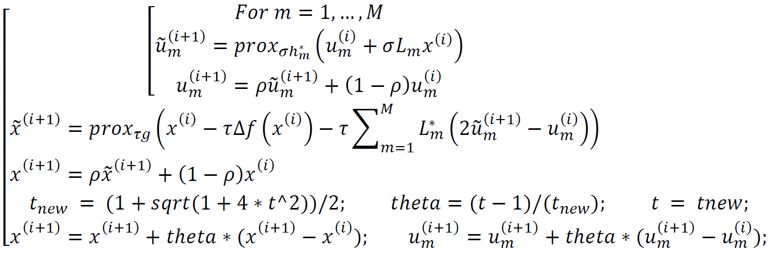
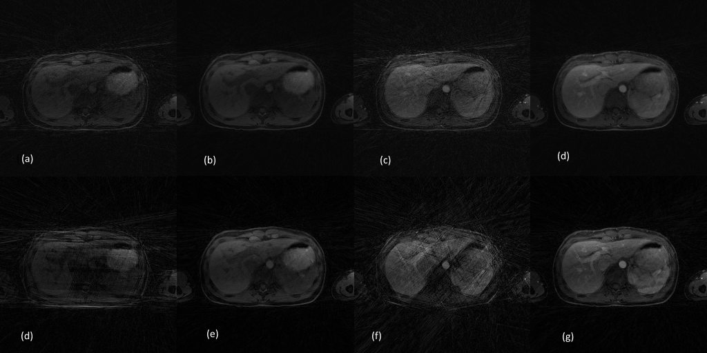
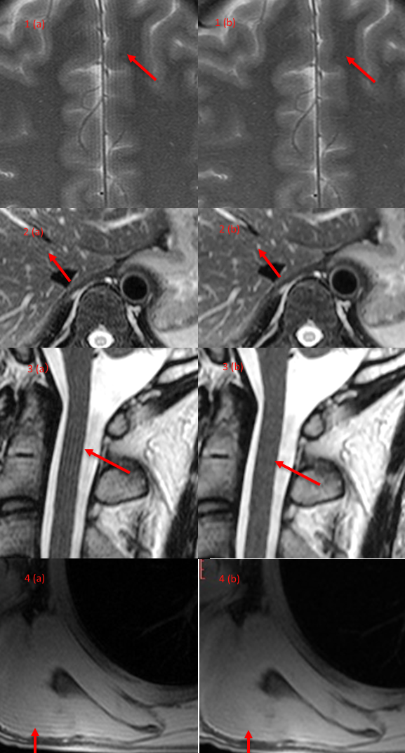
Fig. 3. Truncation artifact
suppression on clinical images. left column is original images, and right column is after processing. (1a, 1b) are brain images, (2a, 2b) are liver images, (3a, 3b) are spinal cord images, and (4a, 4b) are lung images. arrows indicate regions for comparisons.