1421
A novel compressed sensing inspired approach for flow reconstruction1Department of Electrical Engineering, Pontificia Universidad Católica de Chile, Santiago, Chile, 2Biomedical Imaging Center, Pontificia Universidad Católica de Chile, Santiago, Chile, 3Institute for Biological and Medical Engineering, Schools of Engineering, Medicine and Biological Sciences, Pontificia Universidad Católica de Chile, Santiago, Chile, 4Department of Radiology, School of Medicine, Pontificia Universidad Católica de Chile, Santiago, Chile
Synopsis
High scan times are one of the most important drawbacks in 4D flow scans and multiple solutions have been proposed to solve this issue. We propose a novel method for undersampled flow reconstruction inspired on the ideas of compressed sensing. By considering the magnitude and complex phase as separate variables, we were able to impose independent properties on each, such as having a constant magnitude over all flow enconding acquisitions and enforcing low phase values on low magnitude areas, thus directly reducing the resulting images' noise. Our method was able to successfully reconstruct flow data with negligible error from undersampled data.
Purpose
There has been an increasing amount of interest in 4D-flow imaging in the last few years. Unfortunately, its translation to the clinic has been hampered because of the long acquisition times. Fast reconstruction techniques have been proposed to accelerate the acquisition of flow images, either using fast 3D trajectories, like PC-VIPR1, or using undersampled reconstruction techniques, like k-t2 or compressed sensing3,4. A common approach of these methods is to independently reconstruct each velocity segment (with and without bipolar gradient) and then combine them to obtain the final velocity images.
In this work we propose a reconstruction method for undersampled flow data inspired by Compressed Sensing ideas. Our method enforces data consistency in the reconstruction process from all segments at once, as well as from multi-coil data, so that less input data is required, and therefore scan times can be further reduced.
Methods
Considering the magnitude and phase as separate variables in the reconstruction problem allows us to promote distinct structural properties on each. We propose the reconstruction procedure
$$(m^\star, \phi^\star, S^\star) \in \arg\min_{m,\phi,S} f(m,\phi,S) := \sum_{c,r}\dfrac{1}{2}||y^c_r-\mathcal{F}_\Omega(S^c\odot m\odot e^{i\phi_r})||_2^2 + \lambda_m \| W m\|_2^2 + \lambda_S \|WS\|_1 + \lambda_\phi R_\phi(m,\phi)$$
The input data $$$y^c_r$$$ denotes the k-space data for the segment $$$r$$$ and coil $$$c$$$. $$$\mathcal{F}_\Omega$$$ is the Fourier transform applied to points in $$$\Omega$$$. The magnitude $$$m$$$ is assumed to be the same for each segment (4 in 4D flow) and each segment has a different complex phase. Coil sensitivities $$$S^c$$$ are also treated as optimization variables. $$$W$$$ denotes the db4 wavelet transform. All variables are real valued arrays. In particular, we assume the sensitivities are real.
While the squared-norm of the residual promotes data consistency, three regularizers enforce structure in the reconstruction. We considered the squared $$$\ell_2$$$-norm of the db4 wavelet coefficients of the magnitude with $$$\lambda_m = 10^4$$$ in order to regularize without over-smoothing and the $$$\ell_1$$$-norm of db4 wavelet coefficients of the sensitivities with a weight $$$\lambda_S = 10^5$$$ in order to promote smoothness. Finally, we considered a magnitude-dependent weight that enforces small values of the phase when the magnitude is small in order to reduce artifacts in the reconstructed phase where the reconstructed magnitude is small. The regularizer is given by $$R_\phi(m,\phi) = \left\lVert \dfrac{\phi}{1+e^{-a (m_0^2-m^2)}} \right\rVert^2$$ With $$$a=1, m_0=0.1$$$. Although the objective is non-convex, it can be represented as $$$f(m,\phi,S) = g(T(m,\phi,S))$$$ where $$$g$$$ is convex and $$$T$$$ is a smooth non-linear map. Problems of this form can be solved with a Gauss-Newton Trust-Region approach: at each iterate $$$(m_k,\phi_k,S_k)$$$ we minimize a model for $$$f$$$ near the iterate over a $$$\ell_2$$$-trust-region to find the next one. The model is constructed by linearizing $$$T$$$ around the current iterate. This way, each trust-region problem can be solved efficiently with off-the-shelf first-order solvers; we used TFOCS5. To avoid numerical instabilities, only the phase term is linearized for $$$R_\phi$$$.
Results
We tested our algorithm in two data sets acquired in a 1.5T MR Philips Achieva Scanner consisting of 4D flow data acquired in a single sagittal slice of the aorta with parameters FOV=250x250mm, res=2.3x2.3x2.3mm, TR/TE=5/3ms. The data sets were retrospectively undersampled using different factors.
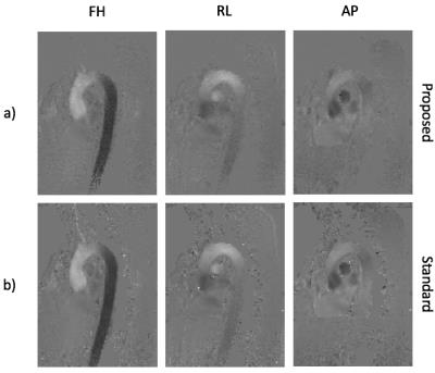
Comparing the result of our undersampled reconstruction method to the fully sampled and post-processed data shows negligible differences as can be appreciated in Figures-1a-b.
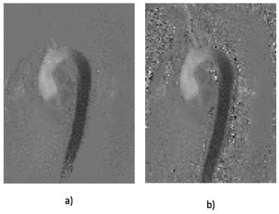
It is worth noting that by using the phase regularizer, post-processing is not needed for velocity data, as it is usually the case for standard flow reconstruction6 (Figure-2).
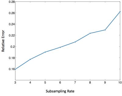
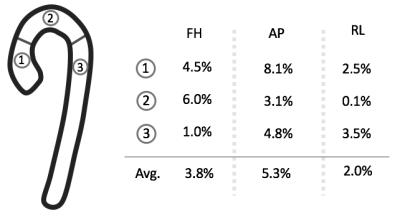
Figure-3 shows the mean reconstruction error by comparing the velocity magnitude of our method for different undersampling factors versus the fully sampled data set. Table-1 in Figure-4 shows quantitative velocity measurements in different sections of the aorta compared with the fully sampled reconstruction. Negligible difference can be observed between our method and the fully sampled reconstruction.
Discussion and Conclusion
We have proposed a novel methodology to reconstruct velocity images from phase contrast acquisition. Both images and numerical data matches the fully sampled reconstructed signal with low error in areas of relevant data. A great advantage of the method is that it does not require to combine phase information from different coils since the phase and magnitude images are independent to the number of coils in the problem formulation. Additionally, since all information from different segments is included, the method directly obtains velocity images for each segment simultaneously. Furthermore, the proposed method is able to successfully separate magnitude and phase signals in the optimization problem which can lead to future studies of the regularizers used for each variable to further improve the reconstruction quality for higher undersampling factors.Acknowledgements
C.SL. was partially funded by the grants Fondecyt de Iniciación 11160728, CONICYT - PIA - Anillo ACT1416 and CONICYT FONDEF/I Concurso IDeA en dos etapas ID15|10284. S.U. was partially funded by the grant Fondecyt 1141036.References
1. Gu, T., Korosec, F. R., Block, W. F., Fain, S. B., Turk, Q., Lum, D., … Mistretta, C. A. (2005). PC VIPR: A high-speed 3D phase-contrast method for flow quantification and high-resolution angiography. American Journal of Neuroradiology, 26(4), 743–749. http://doi.org/26/4/743 [pii]
2. Pedersen, H., Kozerke, S., Ringgaard, S., Nehrke, K., & Won, Y. K. (2009). K-t PCA: Temporally constrained k-t BLAST reconstruction using principal component analysis. Magnetic Resonance in Medicine, 62(3), 706–716. http://doi.org/10.1002/mrm.22052
3. Santelli, C., Loecher, M., Busch, J., Wieben, O., Schaeffter, T., & Kozerke, S. (2015). Accelerating 4D flow MRI by exploiting vector field divergence regularization. Magnetic Resonance in Medicine, 125, 115–125. http://doi.org/10.1002/mrm.25563
4. Lustig, M., Donoho, D., & Pauly, J. M. (2007). Sparse MRI: The application of compressed sensing for rapid MR imaging. Magnetic Resonance in Medicine, 58(6), 1182–1195. http://doi.org/10.1002/mrm.21391
5. Becker, S. R., Candès, E. J., & Grant, M. C. (2011). Templates for convex cone problems with applications to sparse signal recovery. Mathematical Programming Computation, 3(3), 165–218. http://doi.org/10.1007/s12532-011-0029-5
6. Walker, P. G., Cranney, G. B., Scheidegger, M. B., Waseleski, G., Pohost, G. M., & Yoganathan, A. P. (1993). Semiautomated method for noise reduction and background phase error correction in MR phase velocity data. Journal of Magnetic Resonance Imaging: JMRI, 3(3), 521–30. http://doi.org/10.1002/jmri.1880030315
Figures


