1416
Beyond Low-Rank and Sparsity: A Manifold driven Framework for Highly Accelerated Dynamic Magnetic Resonance Imaging1Electrical Engineering, University at Buffalo, State University of New York, Buffalo, NY, United States, 2Biomedical Engineering, University at Buffalo, State University of New York, Buffalo, NY, United States
Synopsis
The state-of-the-art methods in accelerating dynamic Magnetic Resonance (dMR) Imaging rely on sparse and/or low-rank priors. We propose a novel manifold driven framework that exploits the manifold smoothness priors to highly accelerate data acquisition in dMR. We postulate that images in dMR lie on or close to a smooth manifold and learn the manifold geometry from the navigator signals. Capitalizing on the learned manifold, we develop two regularization loss functions and subsequently build a framework to reconstruct dMR images from highly undersampled k-space data. The proposed method is shown to be superior than competitive methods in different data sets.
Purpose
To reconstruct dMR images from undersampled k-space data using nonlinear data-adaptive manifold model, thereby highly accelerating data acquisition in dMR imaging.
Introduction
Reconstruction of dynamic image series $$$\mathbf{X}$$$ from undersampled k-space data involves solving a regularized optimization problem as,
$$\arg\min\nolimits_{\mathbf{X}}\left\|\mathbf{Y}-\mathbf{\phi}(\mathbf{X})\right\|_{\text{F}}^2+\lambda \cal{R}(\mathbf{X}),\quad(1)$$
where $$$N\times N_\text{fr}$$$ Casorati matrix $$$\mathbf{X}=[\mathbf{x}_{1},\mathbf{x}_{2},\ldots \mathbf{x}_{N_{\text{fr}}}],N=N_{\text{p}}\times N_{\text{fr}}$$$, $$$\mathbf{\phi}$$$ is measurement operator, and $$$\mathbf{Y}$$$ is acquired k-space data. While state-of-the-art methods rely on sparse[1,2] and/or low rank[3,4,5] priors, user-defined thus data agnostic manifold model[10] has been recently proposed and shown improvement. In this paper, we propose a more general manifold framework and develop two novel regularization cost functions $$${\mathcal{R}}(\cdot)$$$ based on manifold smoothness.[6,7,8]
Methods
Manifold Learning: Capitalizing on the smoothness of a manifold (Fig.1(a)), we postulate that each image vector $$$\mathbf{x}_i$$$ can be approximated by the affine combination of its neighboring image vectors, mimicking well-known properties of tangent spaces of smooth manifolds.[9] Each image is related to its neighbor by the sparse weight vectors $$$\boldsymbol{\omega}_{i}$$$ such that,$$\boldsymbol{\omega}^{i}\in\underset{\boldsymbol{\omega}_{i}^{H}\mathbf{1}_{N_{\text{fr}}}= 1,\, \omega_{i}^{i}=0}{\operatorname{argmin}}\left\|\mathbf{x}_{i}-\sum\nolimits_{n = 1}^{N_{\text{fr}}} \omega_{i}^{n}\mathbf{x}_n\right\|+\beta\left\|\boldsymbol{\omega}^{i}\right\|_{1}.\quad(2)$$ Here, $$$\mathbf{1}_{N_{\text{fr}}}$$$ is the all-one vector. The constraint $$$\boldsymbol{\omega}_{i}^{H}\mathbf{1}_{N_{\text{fr}}}=1,(\cdot)^{{H}}$$$ denotes Hermitian transposition justifies the affine neighboring relations and $$$\beta ≥ 0$$$ can be tuned to constrain the numbers of neighbors $$$K_{\text{n}}$$$.
Manifold Embedding and Regularization: Having learned the weight matrix $$$\mathbf{W}$$$ with entries $$$\omega_{i}^{n}$$$ using navigator[3] signals, we develop two regularization cost functions that promotes the manifold geometry described by (2).[6,7,8,9] The nonlinear embedding that maps $$$\mathbf{x}_i\in\mathbb{C}^{N}$$$ into $$$\mathbb{C}^{M}$$$ is given by solving$$ \underset{\begin{subarray}{c}\boldsymbol{\Psi}\in\mathbb{C}^{M\times N_{\text{fr}}},\boldsymbol{\Psi} \boldsymbol{\Psi}^{{H}}=\mathbf{I}_M,\,\\\boldsymbol{\Psi}\mathbf{1}_M=\mathbf{0}_M\end{subarray}}{\operatorname{argmin}}\left\|\boldsymbol{\psi}_{i}-\sum\nolimits_{n=1}^{N_{\text{fr}}} \omega_{i}^{n}\boldsymbol{\psi}_n\right\|,\quad (3)$$where $$$\boldsymbol{\Psi} = [\boldsymbol{\psi}_{1}\;\boldsymbol{\psi}_{2}\;\ldots\;\boldsymbol{\psi}_{N_{\text{fr}}}]$$$. The constraint $$$\boldsymbol{\Psi}\boldsymbol{\Psi}^{{H}}=\mathbf{I}_M$$$, where $$$\mathbf{I}_M$$$ is $$$M \times M$$$ identity matrix, excludes trivial all zero solution, whereas $$$\boldsymbol{\Psi}\mathbf{1}_M = \mathbf{0}$$$ centers the columns of $$$\boldsymbol{\Psi}$$$ around $$$\mathbf{0}$$$. The solution of (3) is given by the eigen-decomposition of appropriate $$$N_{\text{fr}}\times N_{\text{fr}}$$$ matrices[6,7] $$$\boldsymbol{\mathcal{K}}:=(\mathbf{I}-\mathbf{W})(\mathbf{I}-\mathbf{W})^{{H}}$$$ and $$$\boldsymbol{\mathcal{L}}:=\mathbf{D}-\mathbf{W}$$$, where $$$\mathbf{D}$$$ is a diagonal matrix with entries $$$d_{ii}:=\sum_{n=1}^{N_{\text{fr}}} \omega_{i}^{n}$$$. Based on these two matrices we develop two regularizers.
$$$\quad\quad$$$A. Regularizer 1 (affine combination) enforces the affine combination modeling assumption such that, $${\mathcal{R}}_{1}(\mathbf{X})=\left\|\mathbf{X}(\mathbf{I}-\mathbf{W})\right\|_{\text{F}}^{2}= \text{tr}(\mathbf{X}\boldsymbol{\mathcal{K}}\mathbf{X}^{{H}}),\quad (4)$$ It should be noted that the $$$i ^{th}$$$ column of $$$\mathbf{X}(\mathbf{I}-\mathbf{W}),$$$ $$${\mathbf{x}}_{\text{err}}^{i}=\mathbf{x}_{i}-\sum_{n=1}^{N_{\text{fr}}}\omega_{i}^{n}\mathbf{x}_{n}$$$ gives the error of approximation for $$$\mathbf{x}_i.$$$
$$$\quad\quad$$$ B. Regularizer 2 (smoothness) The incidence matrix $$$\mathbf{G}^{H} $$$ of a graph $$$\boldsymbol{\mathcal{L}}=\mathbf{G}\mathbf{G}^{{H}}$$$ resembles a finite difference operator such that $$$\left\|\mathbf{X}\mathbf{G}\right\|_F^2$$$ resembles Tikhonov regularization [9,10]. Hence, defining the second regularizer as, $$\mathcal{R}_{2}(\mathbf{X})=\left\|\mathbf{X}\mathbf{G}\right\|_{\text{F}}^{2}=\text{tr}(\mathbf{X}\boldsymbol{\mathcal{L}}\mathbf{X}^{{H}}).\quad(5)$$
The regularizer $$${\mathcal{R}}_2(\cdot)$$$ is similar to the "$$$\ell_2$$$STORM'' reported in[10,7]. While the neighborhoods in [10] are user-defined and thus data-agnostic and prone to model errors, the neighborhoods of the present framework are defined by the data themselves via affine relations defined by (2).
Manifold regularization and reconstruction: The singular vectors of matrices $$$\boldsymbol{\mathcal{K}}$$$ and $$$\boldsymbol{\mathcal{L}}$$$ provide the solutions for (3) and describe the temporal basis of dynamic image series as illustrated in Fig. 1(b). Eigen decomposition has been widely used to learn temporal basis in dMR imaging.[3,4,5] While PCA decomposition preserves the variation of data, decomposition of $$$\boldsymbol{\mathcal{K}}$$$ and $$$\boldsymbol{\mathcal{L}}$$$ preserves the neighborhood relation defined by (2). Let, $$$\boldsymbol{\mathcal{K}}$$$ and $$$\boldsymbol{\mathcal{L}}$$$ have singular value decomposition as $$$\boldsymbol{\Psi}^{{k}} \boldsymbol{\Sigma}^{{k}} {\boldsymbol{\Psi}^{{k}}}^{{H}}$$$ and $$$ \boldsymbol{\Psi}^{{l}}\boldsymbol{\Sigma}^{{l}}{\boldsymbol{\Psi}^{{l}}}^{{H}}.$$$ Substituting them in (4) and (5) respectively, the original problem in (1) boils down to, \begin{align}&\arg\min\nolimits_{\mathbf{U}^{k}} \left\|\mathbf{Y}-\mathbf{\phi}\left(\mathbf{U}^{k} (\boldsymbol{\Psi}^{k})^{H}\right)\right\|_{\text{F}}^2+\lambda\sum\nolimits_{m=1}^{M}\sigma_{m}^{k} \left\|\mathbf{u}_{m}^{k}\right\|^{2},\quad(6)\\&\arg\min\nolimits_{\mathbf{U}^{l}}\left\|\mathbf{Y}-\mathbf{\phi}\left(\mathbf{U}^{l}(\boldsymbol{\Psi}^{l})^{H}\right)\right\|_{\text{F}}^2 +\lambda\sum\nolimits_{m=1}^{M}\sigma_{m}^{l}\left\|\mathbf{u}_{m}^{l}\right\|^{2},\quad(7)\end{align} where $$$\textbf{U}^k=\mathbf{X}\boldsymbol{\Psi}^{{k}} $$$ and $$$\mathbf{u}_{m}^{k}= \mathbf{X}\boldsymbol{\psi}_{m}^{k}$$$ is the projection of $$$\mathbf{X}$$$ on the $$$m^{th}$$$ minor singular vector of $$$\boldsymbol{\mathcal{K}}$$$. Notations in (7) have same meaning as in (6). Finally, conjugate gradient method is used to solve (6) and (7) and reconstruct desired dynamic image series.
Results
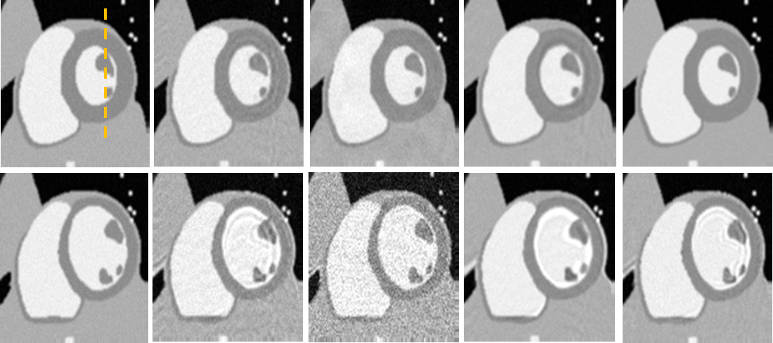
A. Phantom Data[11] Data Parameters: Data Matrix $$$(N_{\text{p}}\times N_{\text{f}}\times N_{\text{fr}})=408\times 408\times 360$$$. Retrospective Cartesian 1D undersampled with about 14 phase encoding lines perframe (4 navigator lines), net reduction factor (R≈30).
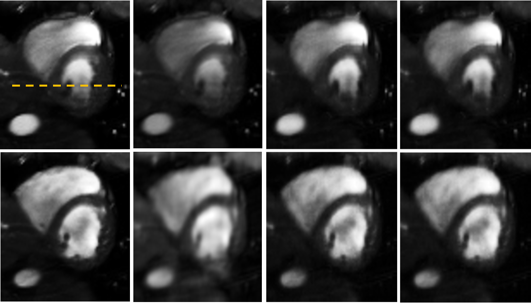
B. Free breathing cardiac cine Data Parameters: $$$(N_{\text{p}}\times N_{\text{f}}\times N_{\text{fr}})=156\times\times 192\times1000$$$, $$$TR/TE=5.84/4$$$ms, $$$\text{FOV}=284\times 350$$$mm, $$$\text{spatial resolution}=1.8$$$mm, $$$\text{Numbers of Channel}=12$$$. Prospective Cartesian 1D undersampled, about 14 phase encoding lines per frame (4 navigator lines), net reduction factor (R≈10).
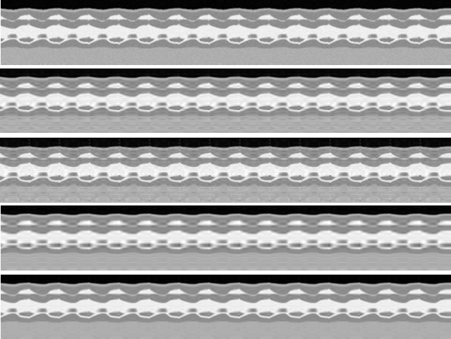
Fig.(2) and Fig.(3) show
the spatial and temporal cross section results for phantom data
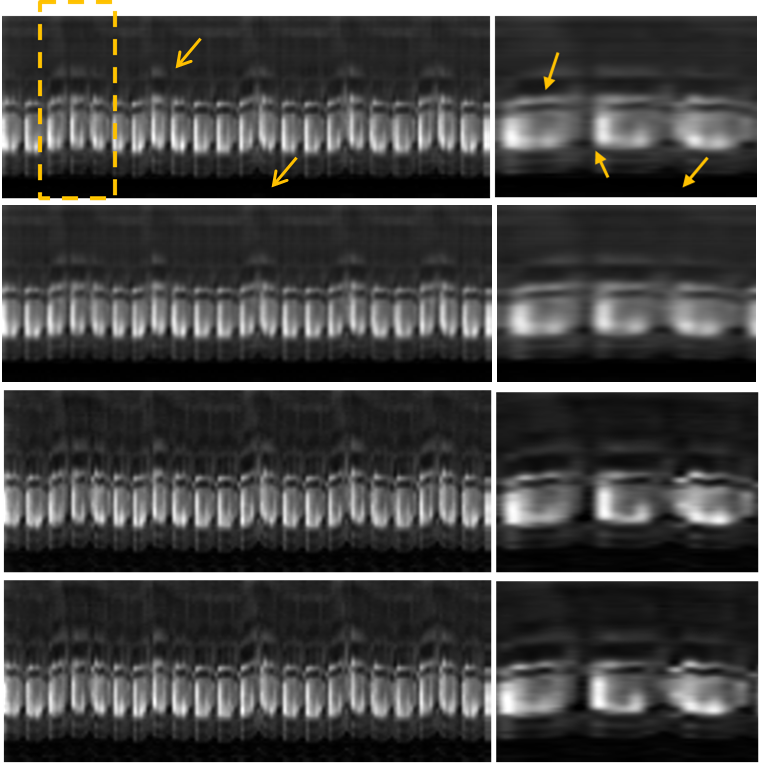
whereas Fig.(4) and Fig.(5) are corresponding to in-vivo data. The
proposed method outperforms the competitive methods. This is also
reflected by the lower error values(RNMSE values in parenthesis). The
PS-sparse method tends to have sharper spatial images in Fig.(4). However,
the temporal details are lost and looks smoother, which might be
the result of over smoothing of temporal basis by low-rank and periodic
assumption.
Conclusion
A novel manifold driven framework for dMRI is developed and its application is verified through numerous experiments. The proposed method is independent of periodic assumption and motivates its usability in many other applications such as dynamic contrast enhanced imaging and speech imaging.Acknowledgements
The authors would like to thanks A.Christodoulou and Z.P. Liang for providing in-vivo data. This work is supported in part by the National Science foundation (NSF) CCF-1514403, NSF 1514056 and the National Institute of Health R21EB020861References
1. M. Lustig, D. Donoho, and J. M. Pauly, “Sparse MRI: The application of compressed sensing for rapid MR imaging,” Magnetic Resonance in Medicine, vol. 58, no. 6, pp. 1182–1195, 2007.
2. D. Liang, E. V. DiBella, R.-R. Chen, and L. Ying, “k-t ISD: Dynamic cardiac MR imaging using compressed sensing with iterative support detection,” Magnetic Resonance in Medicine, vol. 68, no. 1, pp. 41–53, 2012.
3. Z.-P. Liang, “Spatiotemporal imaging with partially separable functions,”in Biomedical Imaging (ISBI), IEEE International Symposiumon, April 2007, pp. 988–991.
4. B. Zhao, J. P. Haldar, A. G. Christodoulou, and Z.-P. Liang, “Image reconstruction from highly undersampled (k,t)-space data with joint partial separability and sparsity constraints,” Medical Imaging, IEEE Transactions on, vol. 31, pp. 1809–1820, 2012.
5. H. Jung, J. C. Ye, and E. Y. Kim, “Improved k-t BLAST and k-tSENSE using FOCUSS,” Physics in medicine and biology, vol. 52,no. 11, p. 3201, 2007.
6. S. T. Roweis and L. K. Saul, “Nonlinear dimensionality reduction bylocally linear embedding,” Science, vol. 290, no. 5500, pp. 2323–2326,2000.
7. M. Belkin and P. Niyogi, “Laplacian eigenmaps for dimensionality reduction and data representation,” Neural computation, vol. 15, no. 6,pp. 1373–1396, 2003.
8. F. R. Chung, Spectral Graph Theory. Regional Conference Series in Mathematics, 1992, no. 92.
9. K. Slavakis, G. B. Giannakis, and G. Leus, “Robust sparse embedding and reconstruction via dictionary learning,” in Information Sciences and Systems (CISS), 47th Annual Conference on, March 2013, pp. 1–6.
10. S. Poddar and M. Jacob, “Dynamic MRI using smoothness regularization on manifolds (SToRM),” Medical Imaging, IEEE Transactions on, vol. 35, no. 4, pp. 1106–1115, April 2016.
11. L. Wissmann, S. Claudio, S. William P, and K. Sebastian, “MRXCAT: Realistic numerical phantoms for cardiovascular magnetic resonance,”Journal of Cardiovascular Magnetic Resonance, vol. 16, no. 1, 2014.
Figures
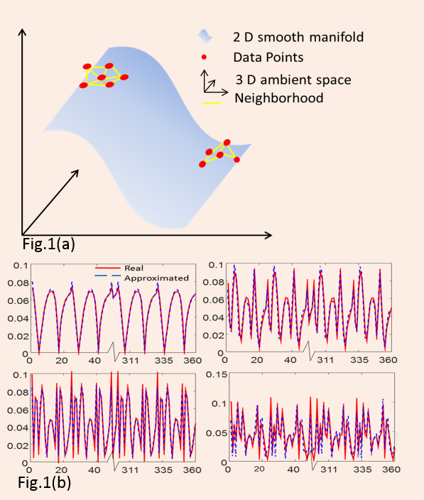
Fig1(a) Illustration of a smooth manifold. 3-dimensional data points lying close to the 2-dimensional smooth manifold surface.
Fig1(b) Real and approximated eigenvectors of $$$\boldsymbol{\mathcal{K}}$$$. Left to right: 2nd, 3rd, 4th and 5th eigenvectors. For better visualization only the section [1:50 311:360] is shown.