1391
Characterising and correcting for MR signal drift in dynamic SPGR oxygen-enhanced MRI acquisitions1Division of Informatics, Imaging and Data Sciences, The University of Manchester, Manchester, United Kingdom, 2CRUK & EPSRC Cancer Imaging Centre in Cambridge and Manchester, Cambridge and Manchester, United Kingdom, 3Division of Molecular and Clinical Cancer Studies, The University of Manchester, Manchester, United Kingdom, 4Department of Radiology, The Christie NHS Foundation Trust, Manchester, United Kingdom, 5Bioxydyn Ltd., Manchester, United Kingdom
Synopsis
Dynamic oxygen-enhanced (OE)-MRI, in combination with dynamic contrast-enhanced (DCE)-MRI, shows use in identifying hypoxic regions in tumours, but relies on an accurate knowledge of baseline (pre contrast-agent administration) tissue characteristics. We present a method of characterising baseline signal drift in an oxygen-enhanced MRI study of preclinical tumour xenografts, where the drift would otherwise impede quantitative analyses. We then demonstrate the utility and necessity of our methods through a comparison of calculated ∆R1 values (reflecting tissue oxygen delivery) with and without our baseline drift correction.
Introduction
Calculation of time-varying relaxation rates in a dynamic MRI study, such as $$$R_1(t)$$$, requires accurate knowledge of the baseline (pre-contrast agent) signal. Drift in the baseline signal that is not appropriately characterised will lead to errors in the calculation of these values, with this effect greatest in low SNR imaging methods, such as oxygen-enhanced (OE)-MRI. Here we show an empirical characterisation of signal drift in an OE-MRI study based on the expected signal change due to $$$B_1$$$ drift and a method for how to use this in the calculation of corrected $$$\Delta R_1(t)$$$ values.Methods
1. Data acquisition
16 preclinical tumours (9 U87 and 7 Calu6 xenografts) were grown in nude mice and underwent OE-MRI imaging using a 7 T Bruker system. Imaging consisted of a variable flip angle (VFA) spoiled gradient echo (SPGR) acquisition to calculate native tissue $$$T_1$$$ ($$$T_{10}$$$) values, followed by a dynamic series of 42 dynamic $$$T_1$$$-weighted SPGR acquisitions at a temporal resolution of 28.8 s, during which the gas supply to the animal was switched from air to oxygen at time point 19.
2. SPGR equation fitting
The SPGR signal equation (Eq. 1)[1] with an exponentially varying flip angle, $$$\alpha(t)$$$, designed to account for $$$B_1$$$ drift (Eq. 2), was fitted to OE-MRI signal data.
$$S(t)=\frac{M_0\sin\left(\alpha(t)\right)\left(1-\exp\left(\frac{-T_R}{T_1}\right)\right)}{1-\cos\left(\alpha(t)\right)\exp\left(\frac{-T_R}{T_1}\right)} \qquad (\textrm{Eq.}1)$$
$$\alpha(t) = (\alpha_0 - \alpha_f)e^{-\gamma t} + \alpha_f \qquad (\textrm{Eq.}2)$$
$$$\alpha_0$$$ and $$$\alpha_f$$$ are the flip angles at the first and last time points of the dynamic series, respectively, and $$$\gamma$$$ is the rate constant of the exponential. $$$\alpha_0$$$ was fixed to the value determined by the automatic scanner calibration, under the assumption that the flip angle set by the scanner is accurate prior to the dynamic series. $$$\alpha_f$$$ was fitted for each tumour on the assumption that the overall degree of drift in flip angle is dependent on the scanner state at the time of scanning, and $$$\gamma$$$ was fitted across the whole tumour cohort on the assumption that any change in $$$\alpha$$$ over time is a machine characteristic.
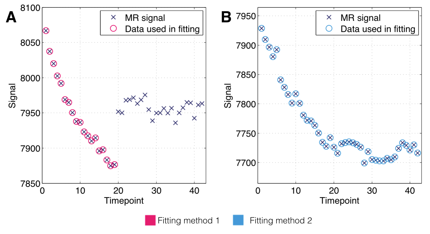
We fitted to 1) pre-oxygen time points for all animals’ tumour voxels, and also to 2) all ‘non-enhancing’ tumour voxels’ full time series, where non-enhancing voxels were located through principal component analysis and Gaussian mixture modelling. The two methods provide a means of cross-validating each other, and the difference in fitting methods is illustrated in Fig. 1.
3. Bootstrap analysis
To evaluate the precision of estimated values of $$$\gamma$$$ and $$$\alpha_f$$$ for both fitting methods, tumour voxels’ enhancement curves were randomly sampled with replacement, within individual tumours, and the SPGR equation fitting was rerun for 1000 bootstrap realisations.
4. Application
Fit values were used to calculate time-varying baseline signal values, $$$S_0(t)$$$, for each tumour voxel by substituting Eq. 2 into Eq. 1. These were then used in Eq. 3 to calculate dynamic $$$T_1(t)$$$ and then $$$\Delta R_1(t)$$$.
$$T_1(t) = \frac{-T_R}{\ln\left(\frac{S_0(t)\cos(\alpha(t)) + (S(t)-S_0(t))\exp\left(\frac{T_R}{T_{10}}\right) - S(t)} {(S_0(t) - S(t))\cos(\alpha(t))-S_0(t)\exp\left(\frac{T_R}{T_{10}}\right) + S(t)\exp\left(\frac{T_R}{T_{10}}\right)\cos(\alpha(t))}\right)} \qquad (\textrm{Eq.}3)$$
Results
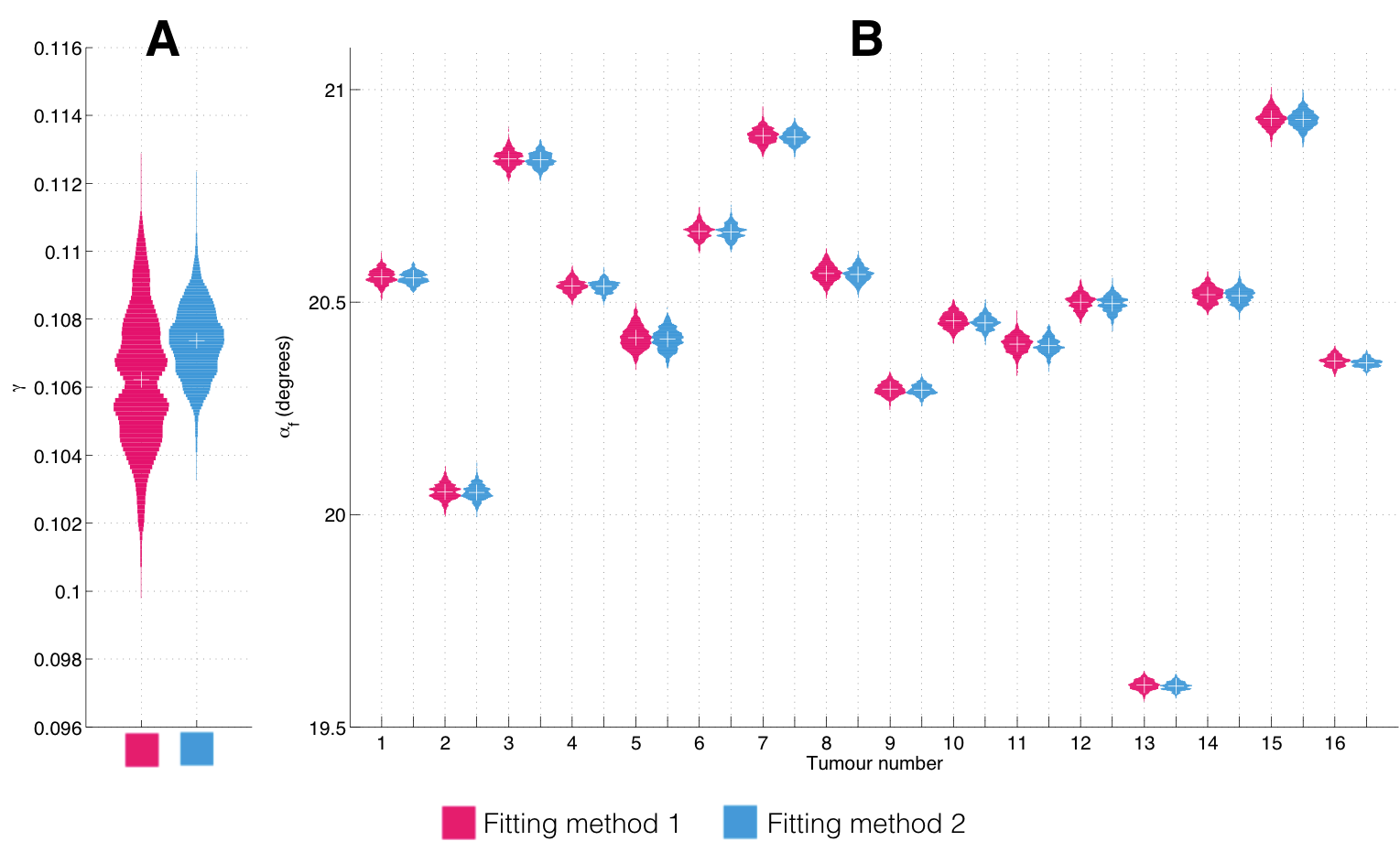
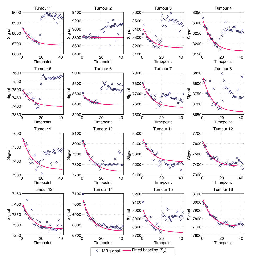
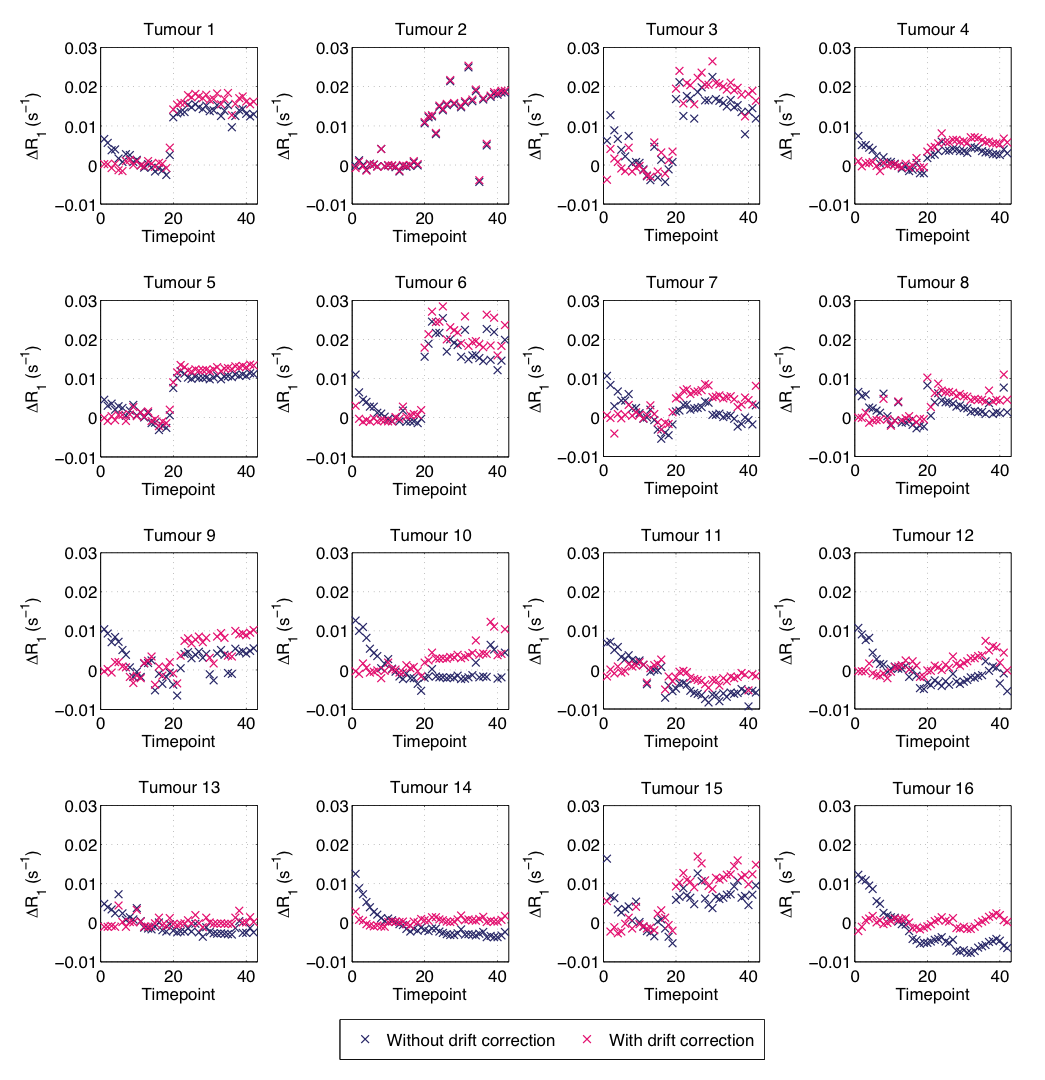
Fig. 2 shows bean plots from the bootstrap analysis, showing mean fit values and precision of $$$\gamma$$$ (Fig. 2A) and $$$\alpha_f$$$ (Fig. 2B) values. Encouragingly, both fitting methods give very similar fit estimates, and so we had confidence in using either. We chose method 1, as this requires fewer assumptions about the data than method 2. Fig. 3 shows the MR signal in each tumour with fitted $$$S_0(t)$$$ curves overlaid, which appear to appropriately characterise the pre-oxygen time points. Fig. 4 shows corresponding $$$\Delta R_1(t)$$$ values calculated using the fitted $$$S_0(t)$$$, and also $$$\Delta R_1(t)$$$ values calculated with no drift correction, illustrating the utility of our methods. Corrected $$$\Delta R_1(t)$$$ values appear physiologically plausible and curves appear drift-free, with the OE-MRI response approximating a step function of different magnitudes, and most tumours showing largely stable values prior to the oxygen switch.Discussion
The choice of an exponential form for $$$\alpha(t)$$$ was made after visual inspection of pre-contrast MR signal values in the tumours (see Fig. 3) and with the hypothesis that some global effect, such as heating in the MRI hardware leading to flip angle variation, was the cause of the signal drift. The high level of precision in the correction parameter estimates and consistency of the drift exponential across tumours is consistent with this hypothesis. Nevertheless, other explanations for the observed drift cannot be excluded.Conclusion
Correction for baseline drift is of particular importance for low contrast-to-noise techniques such as dynamic oxygen-enhanced MRI. The methods presented here appear to effectively remove observed drift, and do so consistently across multiple data sets, suggesting that the methods proposed are both necessary and adequate.Acknowledgements
This is a contribution from the CRUK & EPSRC Cancer Imaging Centre in Cambridge and Manchester (C8742/A18097).References
[1] Fram E K, et al. Rapid calculation of T1 using variable flip angle gradient refocused imaging. Mag Res Imaging. 1987;5:201-8.Figures