Purpose

Myelin-specific imaging is of considerable interest for the detection and monitoring of diseases such as multiple sclerosis. Using a multi-echo spin-echo (MESE) sequence, myelin water fraction (MWF) images have been obtained through multicomponent analysis of T₂ decay using non-negative least squares (NNLS) ¹. However, compared to MESE sequences, multi-gradient recalled echo (MGRE) sequences have the advantage of providing high temporal sampling of the signal decay curve, fast 3D or multi-slice acquisitions, and low SAR. Multicomponent T₂^* analysis is therefore a promising approach to MWF imaging. In this study, we compared MWFs and relaxation times from MGRE and MESE in vivo.

Methods

Measurements were performed on a 3T scanner (Siemens) using a 32-channel head coil. 11 healthy volunteers (aged 18-33 years) were scanned following approval by the local ethics committee and after giving
 informed consent. A single-slice 32-echo MESE sequence was acquired axially: in-plane resolution=1.32x1.32mm², slice thickness=5mm, TR=3000ms, echo spacing (ES)=10ms, bandwidth=260Hz/Px, matrix=192x166, scan time=8min21sec, and SNR(TE1)=470. Following this, a high-resolution 3D T1-weighted scan (MP-RAGE) was acquired. Lastly, a 64-echo MGRE sequence with bipolar readout gradients was acquired: 19 axial slices, in-plane resolution=1.32x1.32mm², slice thickness=2.5mm, TR=2000ms, TE1=2.4ms, ES=1.2ms, bandwidth=1090Hz/pixel, matrix=192x168, flip angle=85⁰, scan time=5min36sec and SNR(TE1)~120. The MP-RAGE images were used for tissue segmentation using FSL FAST ² and the resulting high-resolution tissue masks were resampled to match the resolution of the MGRE and MESE volumes. MGRE magnitude images were smoothed using a non-local means filter ³ and corrected for the effects of field inhomogeneities ($$$\Delta B_{0}$$$) ⁴. Regularized NNLS analysis was performed in white matter (WM) and gray matter (GM) voxels. Maps were generated for the MWF (defined as the sum of components with T₂^*<25ms or T₂<40ms divided by all components) and the geometric mean ⁵ (gm) of the intra/extra-cellular (IE) water relaxation times (gmT_2,IE and gmT^*_2,IE). The multi-slice MGRE-MWF and gmT^*_2,IE maps were resampled to match MESE single-slice volume, to compare the same regions of interest (ROIs) in both MGRE and MESE data sets. ROIs were drawn in four WM structures (genu and splenium of the corpus callosum, minor and major forceps) and six GM structures (caudate nucleus, putamen, thalamus, cingulate gyrus, insular cortex, and cortical GM). For each ROI, the mean MWF, gmT_2,IE, and gmT^*_2,IE were calculated. Two-tailed t-tests, correlation, and Bland-Altman analyses were performed to compare MESE and MGRE-derived measurements.

Results and Discussion

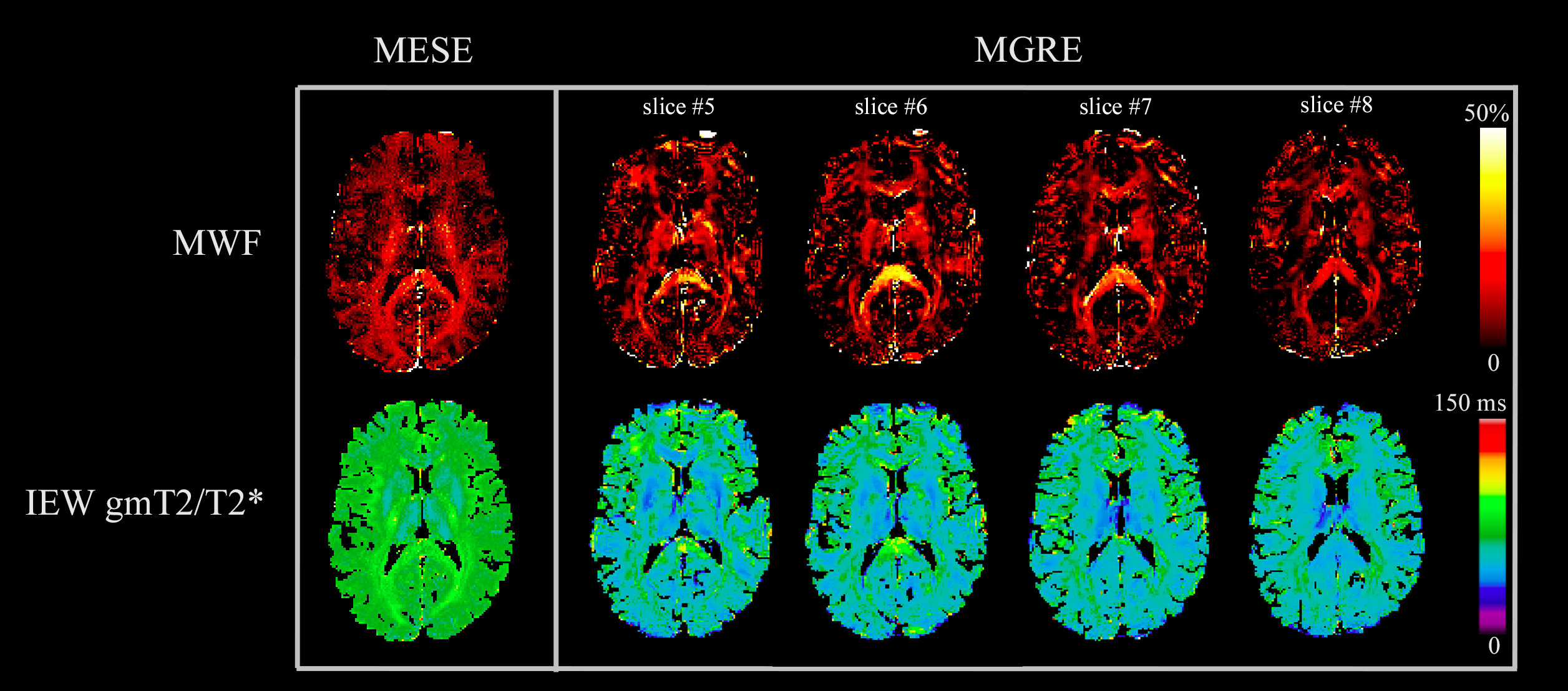
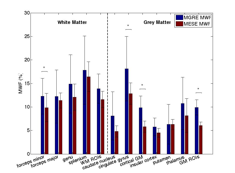
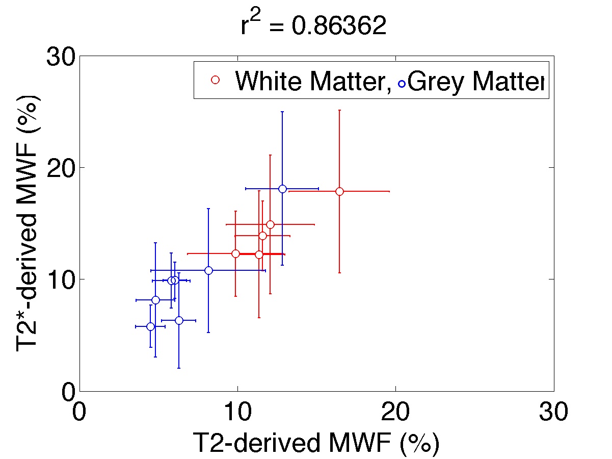
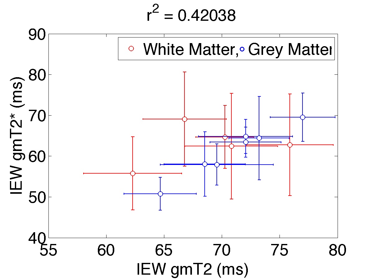
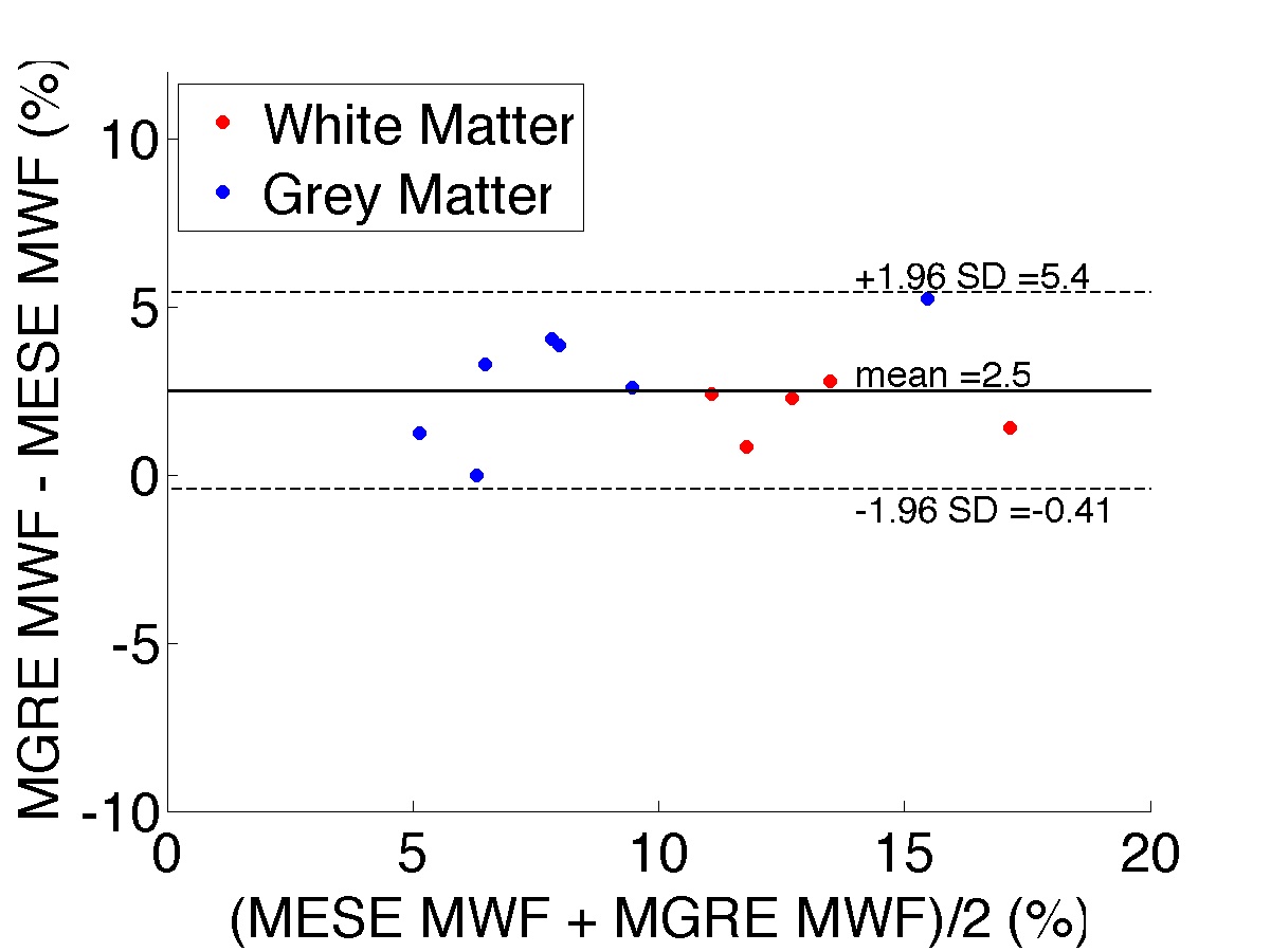
MESE-MWF maps appeared to possess superior image quality compared to MGRE-MWF maps, whereas gmT_2,IE and gmT^*_2,IE maps had comparable image quality (Figure 1). MESE-MWF values were in agreement with previous MESE-MWF studies ⁶ and MGRE-MWFs and MESE-MWFs (averaged over 11 volunteers) were not significantly different in 4 out of 5 WM ROIs, and in 4 out of 6 GM ROIs (two-tailed t-test with p < 0.05) (Figure 2). The only WM ROI where the MWF was significantly different between the two techniques was the forceps minor. We attribute this to its proximity to the nasal sinuses, which lead to large field gradients. Although the correction algorithm largely compensates for the signal loss caused by $$$\Delta B_{0}$$$ in this area, some error may remain. The average (± standard deviation) WM MGRE-MWF was (14±3)%, and not significantly different from the average WM MESE-MWF, (12±2)%. In contrast, the average GM MGRE-MWF (10±2)% was greater than the average GM MESE-MWF (6±1)%. A very strong correlation (r²=0.86) was observed between MGRE and MESE MWFs and a moderate correlation (r²=0.42) was found between gmT_2,IE and gmT^*_2,IE values (Figures 3 and 4). Lastly, a Bland-Altman plot of the MGRE- vs. MESE-MWF (Figure 5) indicates that the MGRE-MWF had a small positive bias of (2.5±1.5)%, with the differences being scattered around the bias with no obvious pattern.

Conclusions

We observed good, but not ideal, correspondence between the two methods. This was mainly due to a lack of agreement between average GM MWFs and a moderate correlation between relaxation times. However, the overall comparison between the two techniques indicated that the MGRE-approach is highly promising, and may be a strong alternative to the MESE technique. Furthermore, the time devoted to sampling the decay curve is shorter in MGRE (78ms in this experiment) than in MESE (320ms), potentially rendering the MGRE method less sensitive to water exchange effects. Additional research to evaluate the repeatability of the MGRE method, and a rigorous assessment of its ability to detect demyelination in MS is warranted.

Acknowledgements

This study was supported by the Fonds de recherche du Québec – Nature et technologies (FRQNT), CREATE Medical Physics Research Training Network grant of the Natural Sciences and Engineering Research Council (NSERC, Grant number 432290), and the Canadian Institutes for Health Research (CIHR - FRN 43871).

References

1. Whittall, K. and A. MacKay, Quantitative interpretation of NMR relaxation data. Journal of Magnetic Resonance (1969), 1989. 84(1): p. 134-152.

2. Zhang, Y., M. Brady, and S. Smith, Segmentation of brain MR images through a hidden Markov random field model and the expectation-maximization algorithm. IEEE Trans Med Imaging, 2001. 20(1): p. 45-57.

3. Coupe, P., et al., An optimized blockwise nonlocal means denoising filter for 3-D magnetic resonance images. IEEE Trans Med Imaging, 2008. 27(4): p. 425-41.

4. Alonso-Ortiz, E., et al., Field inhomogeneity correction for gradient echo myelin water fraction imaging. Magn Reson Med, 2016.

5. Bjarnason, T., Proof that gmT2 is the reciprocal of gmR2. Concepts Magn. Reson., 2011. 38A(3): p. 128-131.

6. Alonso-Ortiz, E., I.R. Levesque, and G.B. Pike, MRI-based myelin water imaging: A technical review. Magn Reson Med, 2014.